Sample Rate Conversion

Objectives

1. Learn about compression and expansion operations on discrete-time signals.
2. Learn about downsampling and upsampling operations on discrete-time signals.
3. Observe the effects of compression and expansion in the time and frequency domains.
4. Gain some experience designing filters and applying them to signals.

Mathematical Background

In class we have derived formulas for sampling and reconstruction and downsampling and upsampling. These derivations and visualizations are available in these slides. (See also these slides.) Here are slide summaries (math and diagrams) for the four operations.

• Sampling (without antialias filter)
• Downsampling (without antialias filter)
• Reconstruction (with ideal low pass filter)
• Upsampling (with ideal low pass filter)

We summarize these formulas here.

Sampling at $F_s=\frac{1}{T}$$F_s = \frac{1}{T}$:

Downsampling at $f_s=\frac{1}{D}$$f_s = \frac{1}{D}$:

Note the strong resemblance between these formulas. There are two main differences.

1. The first difference is explicit: the summation limits in CT sampling formulas are infinite, the summation limits in DT downsampling are finite, and the sample interval $T$$T$ [seconds] is replaced by the downsample interval $D$$D$ [samples].
2. The second difference is implicit: $X(F)$$X(F)$ is aperiodic whereas $X(f)$$X(f)$ is periodic with period 1.

The formulas for reconstruction and upsampling are summarized here.

Reconstruction at $F_s=\frac{1}{T}$$F_s=\frac{1}{T}$:

Upsampling at $f_s=\frac{1}{U}$$f_s = \frac{1}{U}$:

Note the strong resemblance between these formulas. The main difference is the periodic nature of the discrete-time spectra.

Sample Rate Conversion

A sample rate conversion system is shown below. It consists of an upsampling stage (consisting of a $U$$U$-fold expander followed by a low pass filter) in series cascade with a downsampling stage (consisting of a low pass filter followed by a $D$$D$-fold compressor). The low pass filters of the upsampling and downsampling stages have been combined into a single low pass filter with frequency response $H(f)$$H(f)$. The cutoff frequency of this filter is the minimum of $\frac{1}{2U}$$\frac{1}{2U}$ and $\frac{1}{2D}$$\frac{1}{2D}$.

Observation 1: If the input $x[n]$$x[n]$ to this system is sampled at a rate of $F_s$$F_s$ samples/second, then the output $y[n]$$y[n]$ will have a sample rate of $\frac{U}{D}{F}_s$$\frac{U}{D} F_s$. By a suitable selection of $U$$U$ and $D$$D$ (which must positive integers), the sample rate may be changed by any rational factor (at least in theory).

Observation 2: Now suppose the input is $x[n]=\cos (2\pi f_{0}n)$$x[n] = \cos(2\pi f_0 n)$ where $f_0<min(\frac{1}{2U},\frac{1}{2D})$$f_0< \min\left(\frac{1}{2U}, \frac{1}{2D}\right)$. After $U$$U$-fold expansion, the frequency moves to $f_0/U$$f_0/U$. It survives the low pass filter and then maps to $\frac{D}{U}{f}_0$$\frac{D}{U} f_0$ after $D$$D$-fold compression so the output signal is $y[n]=\cos \left(2\pi \frac{D}{U}{f}_{0}n\right)$$y[n] = \cos\left(2\pi \frac{D}{U}f_0 n\right)$.

Observation 3: Notice that the scale factor $\frac{D}{U}$$\frac{D}{U}$ for frequency mapping is the reciprocal of the scale factor $\frac{U}{D}$$\frac{U}{D}$ for sample rate mapping. This is as it must be because the actual frequency of the signal at the input is $F_0=f_0{F}_s$$F_0 = f_0 F_s$ Hz, and the actual frequency of the signal at the output is $F_0=\left(\frac{D}{U}{f}_0\right)\left(\frac{U}{D}{F}_s\right)=f_0{F}_s$$F_0 = \left(\frac{D}{U} f_0\right) \left(\frac{U}{D} F_s\right) = f_0 F_s$ Hz, which his the same frequency at input as at output.

Multistage Sample Rate Conversion

Design a system that converts a signal $x[n]$$x[n]$ with sample rate $F_x=11025$$F_x = 11025$ S/s to a signal $y[n]$$y[n]$ with a sample rate of $F_y=8000$$F_y=8000$ S/s. Using the sample rate conversion system from above we have:

Solving for $D/U$$D/U$ we obtain

Using $U=320$$U=320$ and $D=441$$D=441$ in a single sample rate conversion stage is challenging for several reasons. First the filtering operation must be performed at $U=320$$U=320$ times the input sample rate. That's a massive computational load. Furthermore, the filter design specification has an impossibly tight specification which would require an extremely long filter. Attempting to change the sample rate using a single stage results in a very complex problem. The numbers $441$$441$ and $320$$320$ may be factored into products of small primes suggesting that the sample rate may be converted using a series of five stages with rather low complexity. The assignment is to implement these five sample rate conversion stages. For each stage, use the low pass filter with the trapazoidally shaped magnitude response that we used in CA2.

Illustration

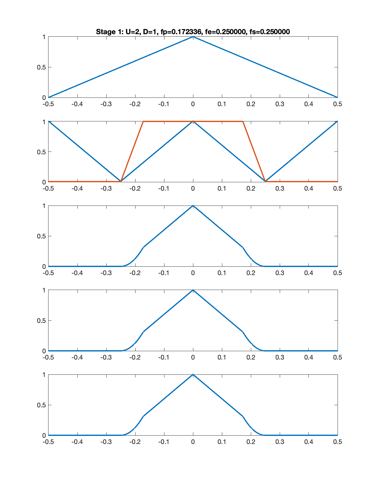
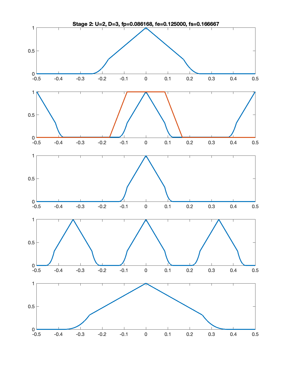
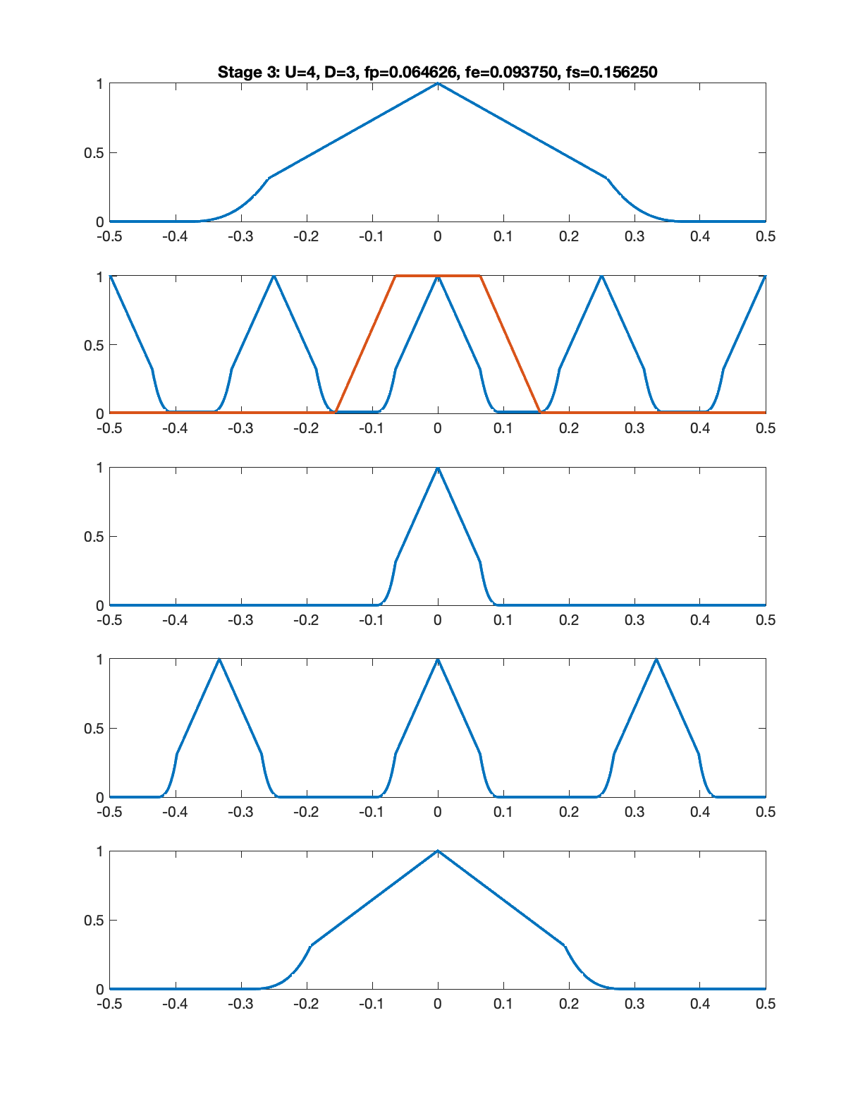
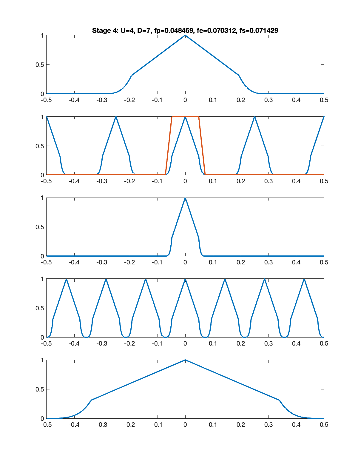
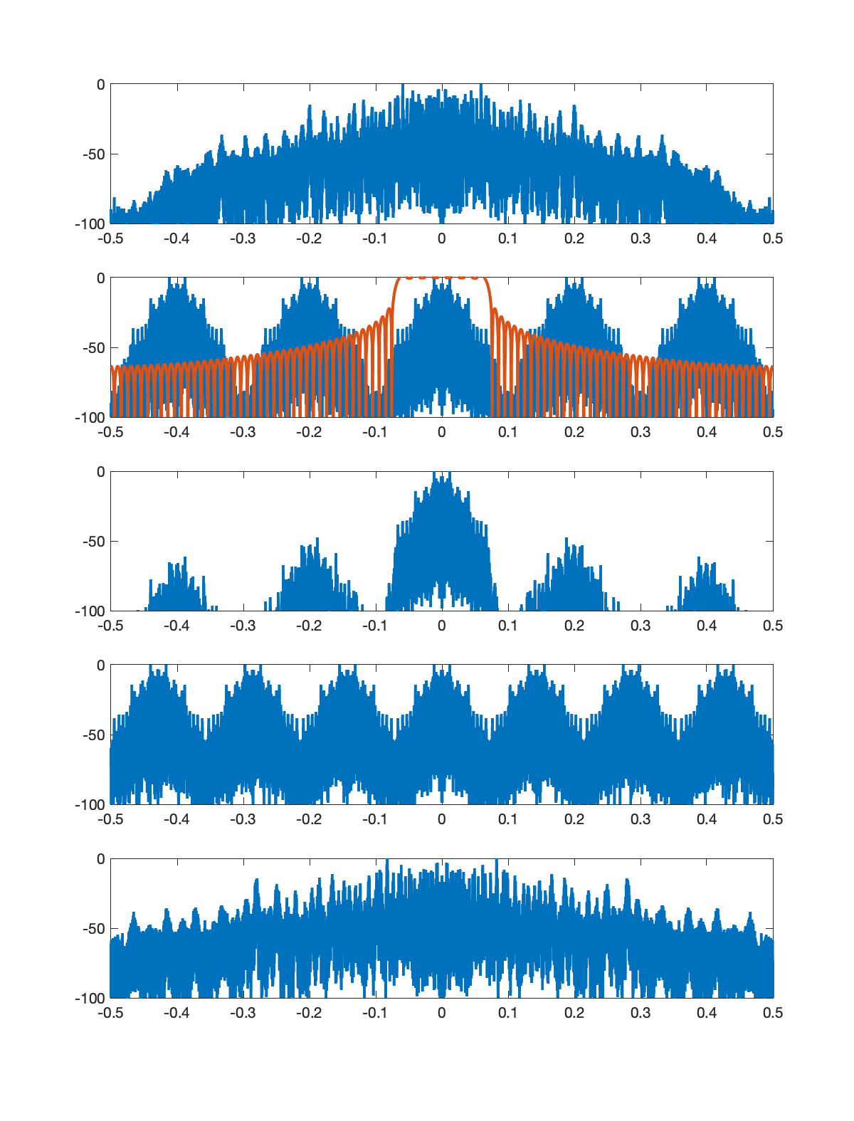
The figures below illustrate the signal spectrum for each of the five stages. In each figure, there are five subplots as follows.

1. Spectrum of the signal input to that stage.
2. Spectrum of the upsampled signal along with the magnitude response of the low pass filter.
3. Spectrum of the signal at the output of the low pass filter.
4. Spectrum of the aliased signal (aliasing formula = replication).
5. Spectrum of the signal output from that stage (downsampling formula = frequency scaling).

Note: In each figure, the title shows the upsampling factor $U$$U$, the downsampling factor $D$$D$, the pass band and stop band edge frequencies $f_p$$f_p$ and $f_s$$f_s$.

Note: In the example below, I assumed that the input signal had a triangular shaped spectrum.

Stage 1: U=2, D=1

Stage 2: U=2, D=3

Stage 3: U=4, D=3

Stage 4: U=4, D=7

Stage 5: U=5, D=7

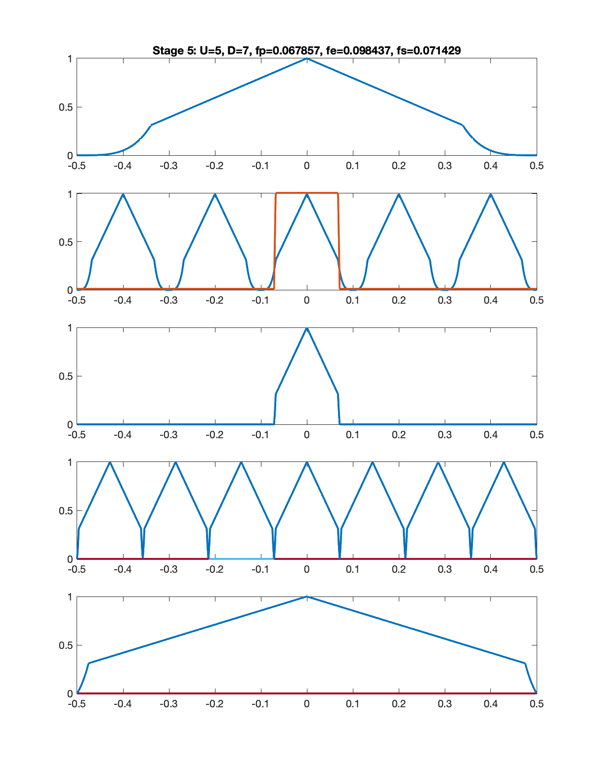
Notice the small amount of aliasing present in the final stage. This occurs because the low pass filter had a stop band edge frequency of $f_s=0.101562$$f_s = 0.101562$, but to avoid aliasing it should have been $f_s=\frac{1}{2D}=\frac{1}{14}=0.0714$$f_s = \frac{1}{2D} = \frac{1}{14} = 0.0714$. This would be a small change to make. Aliasing was avoided in all prior stages.

I performed five stages of sample rate conversion on an audio signal sampled at $11025$$11025$ S/s resulting an an audio signal sampled at $8000$$8000$ S/s. The spectral plots are shown below in dB scaling.

Stage 1: U=2, D=1

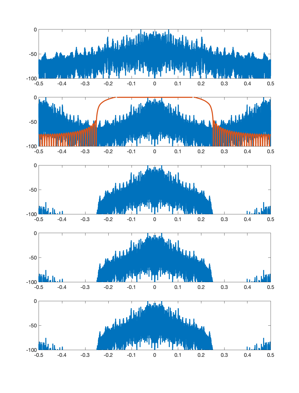
Stage 2: U=2, D=3

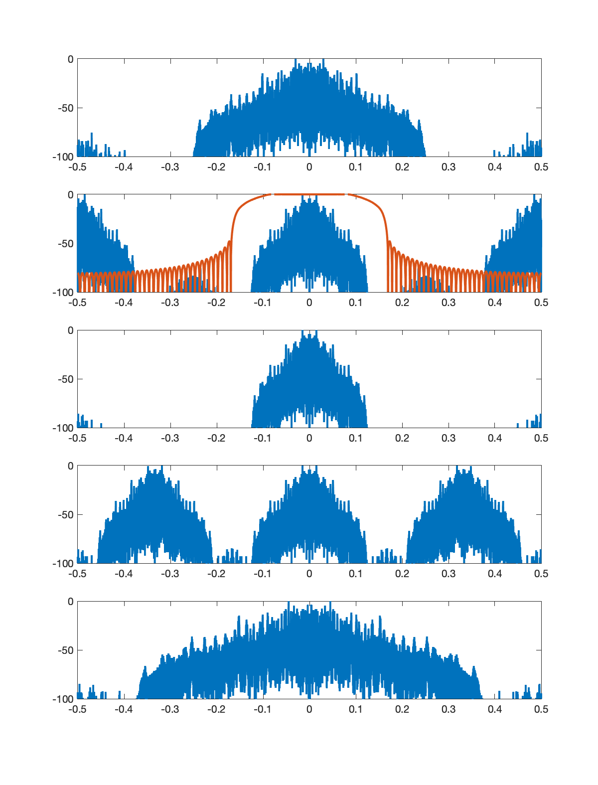
Stage 3: U=4, D=3

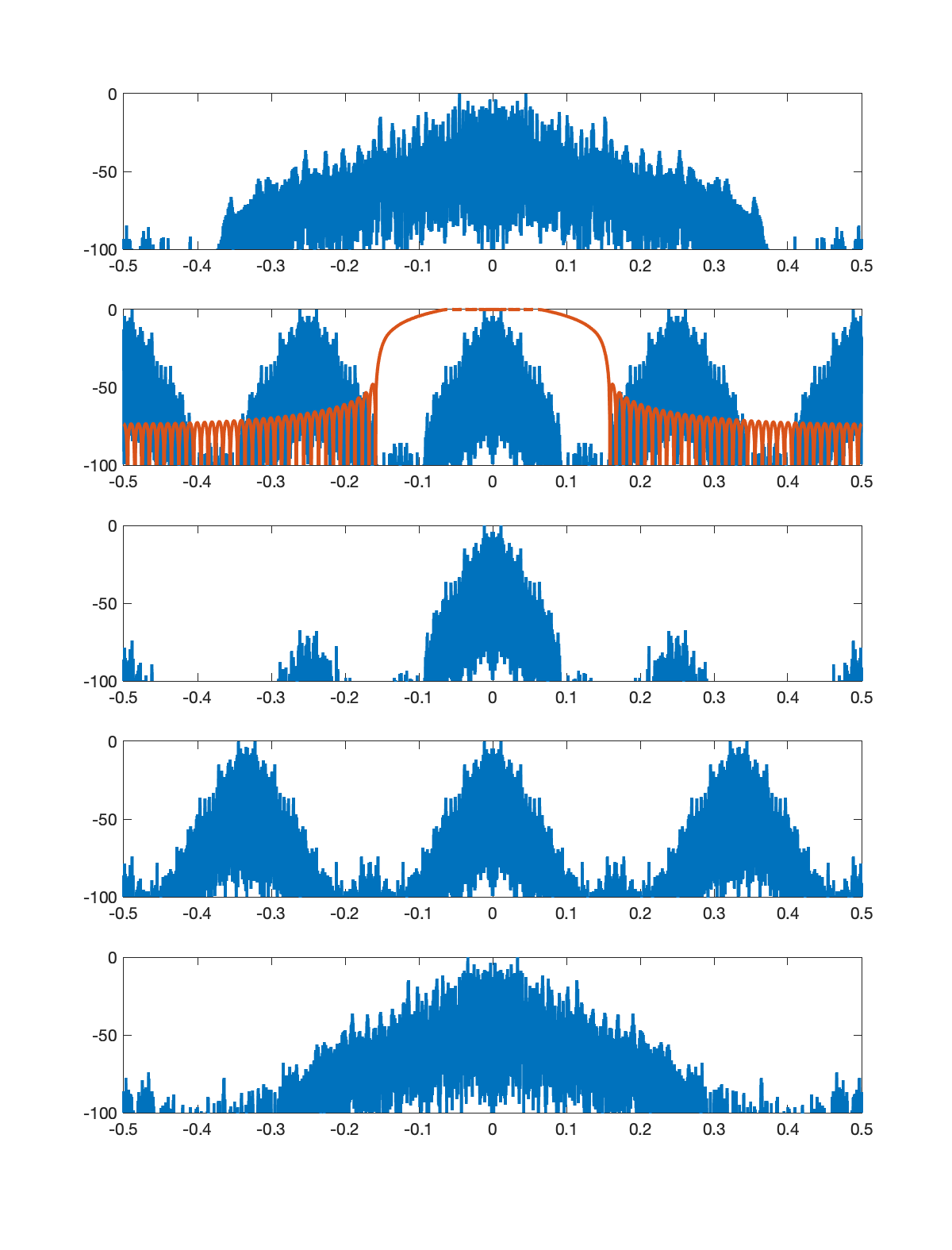
Stage 4: U=4, D=7

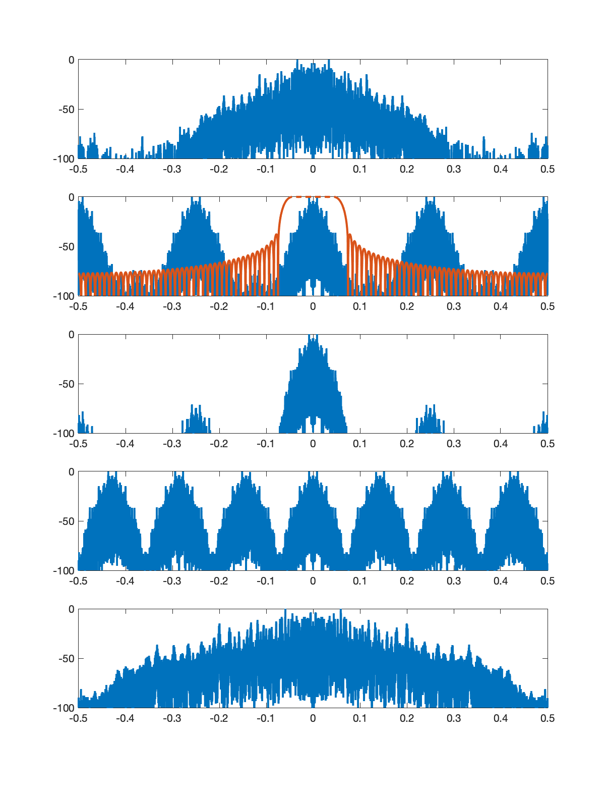
Stage 5: U=5, D=7

Designing Filters

The tricky part of sample rate conversion is designing the filters. Let's figure this out.

There are three frequencies that we have to keep track of in each stage of sample rate conversion. These are as follows.

• $f_p$$f_p$ the pass band edge frequency in the input signal for that stage. Frequencies in the band $|f|\le f_p$$|f|\leq f_p$ must be protected from aliasing and should be free attenuation free.
• $f_m$$f_m$ is the maximum frequency in the input signal for that stage. Frequencies in the band $f_p<|f|\le f_m$$f_p < |f| \leq f_m$ can be attenuated. These are "don't care" frequencies. We have to keep track of $f_m$$f_m$ because we want to avoid aliasing, and if aliasing is going to occur, then it will happen due to energy in the signal at frequencies up to $f_m$$f_m$.
• $f_s$$f_s$ is the stop band frequency of the low pass filter $H(f)$$H(f)$. This frequency will be chosen either to remove images resulting from $U$$U$-fold expansion in which case $f_s=(1-f_m)/U$$f_s = (1-f_m)/U$, or it will be chosen to suppress aliasing before $D$$D$-fold compression in which case $f_s=1/2D$$f_s = 1/2D$. In general, we will let

Consider a general sample rate conversion stage with $U$$U$-fold expansion and $D$$D$-fold compression. The $U$$U$-fold expander maps the following critical frequencies:

The filter $H(f)$$H(f)$ is designed to pass frequencies below $f_p^{\prime }$$f_p'$ and stop frequencies above $f_s$$f_s$, where $f_s$$f_s$ is chosen to suppress either images or aliasing. The maximum frequency at the output of the filter is either $f_m^{\prime }$$f_m'$ or $f_s$$f_s$, whichever is smaller,

Finally, after $D$$D$-fold compression the output pass and maximum frequencies are given by:

Let's apply these ideas to our problem. First we have to make some design decisions. Note that the final sample rate is 8000 S/s and the highest frequency that can be represented at 8000 S/s is half the sample rate or 4000 Hz. We have to provide a transition band for filtering and I'm willing to allow some attenuation of signals above 3800 Hz. I'm going to design the processing to preserve all frequencies below 3800 Hz as alias free and attenuation free. This will be the passband edge frequency throughout all the processing stages. At the input, the normalized version of 3800 Hz is $f_p=3800/11025=0.3447$$f_p = 3800/11025 = 0.3447$ cycles/sample. The maximum frequency at the input is half the sample rate, so $f_m=0.5$$f_m = 0.5$ cycles/sample.

Next consider the first stage with parameters $U=2,D=1$$U=2, D=1$. First map the critical frequencies corresponding to $U=2$$U=2$ fold expansion.

We can see that the filter $H(f)$$H(f)$ should have a passbands edge frequency of 0.1723 cycles/sample and a stop band edge frequency of 0.25 cycles/sample. The filter is designed to reject images.

The critical frequencies in the filter output are

Finally, after $D=1$$D=1$ fold compression, the critical frequencies at the output of this stage are the same

Now we are ready to apply these principles to the subsequent stages.

Assignment

1. Draw a block diagram of the five stage sample rate conversion system that converts from $F_x=11025$$F_x = 11025$ S/s to $F_y=8000$$F_y = 8000$ S/s.
2. Label the block diagram to indicate the sample rate at the output of each block in the system diagram.
3. Suppose the input signal contains a signal at normalized frequency $f_0=1000$$f_0=1000$ Hz. Label the block digram to indicate the frequency of this signal at the output of each block in the system diagram.
4. Write a Matlab function that performs one stage of sample rate conversion (SRC). The signature of the function should be:

xxxxxxxxxx
[y,fp,fm,Fs] = src(x,fp,fm,U,D,Fs)

where $x$$x$ is the input signal, $f_p$$f_p$ is the pass band edge frequency for the input signal, $f_{\text{max}}$$f_\text{max}$ is the maximum frequency in the input signal, $U$$U$ and $D$$D$ are the upsampling and downsampling factors, $F_s$$F_s$ is the input sample rate, and $y$$y$ is the output signal. Note that $f_p,f_m,F_s$$f_p, f_m, F_s$ are all input and output variables. The output frequencies should be scaled $D/U$$D/U$ by the input frequencies and the output sample rate $F_s$$F_s$ should be scaled $U/D$$U/D$ by the input sample rate.

Your function should design and do all the processing for the sample rate conversion for that one stage.

Your function should make plots like those shown above.

5. Call your function five times to perform the five stage sample rate conversion on this audio file.
6. Turn in your plots of the signal spectra for each stage.
7. Turn in a table showing the calculation of the critical frequencies $f_p,f_m$$f_p, f_m$ and $f_s$$f_s$ for each stage.
8. Include a spectrogram plot of the input signal and the final output signal.
9. Turn in your code.