Filtering Lab

Video

Slides

Introduction

In this assignment you will write a custom filtering function in Matlab and use it to process signals through filters (linear, time-invariant, causal, stable systems). You will implement both finite and infinite impulse response filters (both FIR and IIR). The $z$$z$-transform is needed to fully understand the structure and design of these types of systems. However, filtering is a time-domain operation and programs that implement filtering are based on the input-output relationship expressed in the time domain.

From a numerical point of view, the terms convolution and filtering both refer to processing a signal through a linear, time-invariant (LTI) system. The key difference between the operations of convolution and filtering is the time when the samples of the input signal are available. In convolution, all samples of the input signal are assumed known and available at the time the convolution is computed and convolution produces all the samples of the output signal. Convolution is a array-in/array-output computational process. Filtering processes the input signal samples one at a time and produces the output samples one at a time. Thus filtering is appropriate for real-time deployments of LTI systems. Filtering is a sample-in/sample-out computational process.

Objectives

1. Implement FIR filter function and use it to apply filters to signals. Design various types of filters.

   • Design trapazoidal low-pass filters.
   • Construct other types of filters using basic LPFs.
   • Plot magnitude frequency responses using freqz.

2. Implement IIR filter function and use it to apply filters to signals. Design various types of filters.

   • Butterworth and elliptic filters.
   • Notch filters to remove notes or pass only notes (fireflyintro.wav)
   • Plot magnitude frequency responses using freqz.

Difference Equations

Difference equations provide a general description of the input-output relationship for LTI systems in the time-domain. If the input and output are given by $x[n]$$x[n]$ and $y[n]$$y[n]$, respectively, the difference equation for an LTI system has the form

where $a[n]$$a[n]$ and $b[n]$$b[n]$ are the filter coeficients, which are obtained through through a filter design process based on a desired filter specification. Filter design will be discussed elsewhere. For now, suppose that the filter coefficients and the input $x[n]$$x[n]$ is given, and let's focus on how to compute the output $y[n]$$y[n]$.

Before moving on, observe that the left and right-hand sides of $(1)$$(1)$ have the form of convolution and could be rewritten as,

Thus, the most general form of an LTI systems equates the convolution of input and output with two other fixed sequences.

"Solving" the difference equation is how the output is computed. To illustrate the process, let us consider the special case where $N=M=3$$N=M=3$. Then the sums in $(1)$$(1)$ may be expanded as

We generally assume $a[0]=1$$a[0] = 1$ and if this is not the case, then divide both sides by $a[0]$$a[0]$ so that

Now solve for $y[n]$$y[n]$

We see that the output $y[n]$$y[n]$ at the current time depends on the current and past inputs $x[n],x[n-1],x[n-2]$$x[n], x[n-1], x[n-2]$ and past outputs $y[n-1],y[n-2]$$y[n-1], y[n-2]$. Given initial conditions $x[-1],x[-2],y[-1],y[-2]$$x[-1], x[-2], y[-1], y[-2]$, the recursive relation in $(2)$$(2)$ defines the necessary arithmetic needed to compute the output sequence $y[n]$$y[n]$ for $n\ge 0$$n \geq 0$. Generally the initial conditions are assumed to be zero. This amounts to assuming that both $x[n]$$x[n]$ and $y[n]$$y[n]$ are causal sequences.

These same steps can be followed for the general case and we may solve $(1)$$(1)$ for $y[n]$$y[n]$ to obtain the recursive form

where we assume zero initial conditions $x[-1]=\cdots =x[M-1]=y[-1]=\cdots =y[N-1]=0$$x[-1]=\cdots=x[M-1]=y[-1]=\cdots=y[N-1]=0$. Equation $(3)$$(3)$ gives the general form of the difference equation for an IIR filter. An IIR filter function uses a pair of loops to accumulate the products shown in $(3)$$(3)$.

The first summation in $(3)$$(3)$ is the feed forward term as it describes how the input $x[n]$$x[n]$ contributes to the output. The second summation in $(3)$$(3)$ describes how previous outputs feedback and contribute to the current output. An FIR filter has the feed forward term but no feedback,

We see that the $b[k]$$b[k]$ coefficients for an FIR filter are it's impulse response. For IIR filters, the impulse response is a complicated function of both $a[n]$$a[n]$ and $b[n]$$b[n]$ coefficients.

FIR Filters

Your job is to write a Matlab function that implements an FIR filter. There are two inputs: (1) an array $\mathbf{b}=[b[0],b[1],\cdots ,b[M-1]]$$\mathbf{b} = [b[0], b[1], \cdots, b[M-1]]$, and (2) $x[n]$$x[n]$ the current sample of the input signal. The output is $y[n]$$y[n]$, the current output sample.

The function must manage a buffer of internal memory to hold the current and past samples of the input signal in order to compute the current sample $y[n]$$y[n]$ of the filter output.

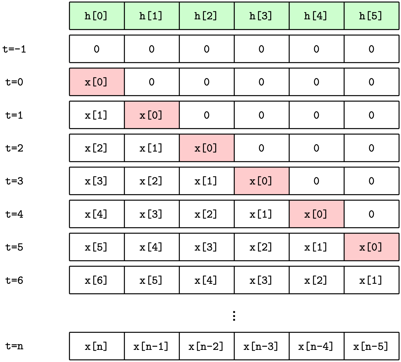
The table above illustrates the movement of data over time through the internal memory of the FIR filter. The top row of the filter contains the impulse response sequence $h[n]$$h[n]$. In this case, the filter order is $M=6$$M=6$. The other rows of the table illustrate how the samples of the input signal shift across the memory buffer. At time $n=-1$$n=-1$, the memory is all zero corresponding to the assumption of a causal input signal. At time $n=0$$n=0$, the first sample $x[0]$$x[0]$ shifts into the buffer. At time $n=1$$n=1$, we see $x[1]$$x[1]$ enter the buffer, but before writing in the new sample, the other samples shift to the right. This process continues at each time step: (1) right-shift previous data, and (2) write in the new sample. At any point in time, the memory buffer contains the current and previous $M-1$$M-1$ input samples. The filter output in $(4)$$(4)$ is computed by multiplying the impluse response buffer (in the first row of the table) with the data memory buffer and summing to produce the output $y[n]$$y[n]$.

A Matlab function that performs filtering must implement the movement of data through a memory buffer as described above. In Matlab, the "persistent" keyword may be used inside a function to create a local variable that persists across subsequent calls to the function. An example appears below.

function y = myFIRfilter(b,x)
persistent z; % Persistent internal filter memory
if isempty(z)
    z = zeros(size(b)); % Initialize to zero
end

% Inputs
% b = [b[0], b[  1], b[  2], b[  3]]
% x = x[n] = the current input sample

% Internal memory before this function call
% z = [x[n-1], x[n-2], x[n-3], x[n-4]]
% Internal memory after this function call
% z = [x[n  ], x[n-1], x[n-2], x[n-3]]

% Shift data in buffer and write in the new input sample
... % Right shift buffer
... % Put new input sample into the buffer

% Compute the filter output
y = ... % Point-by-point multiply and accumulate

Your assignment is to finish writing the myFIRfilter function. Do not use built-in functions or vector operations.Use for loops where needed.

IIR Filters

IIF filters implement the difference equation in $(3)$$(3)$ including both the feedforward and feedback sums. For convenience, equation $(3)$$(3)$ is repeated here along with the special case $N=M=2$$N=M=2$ which we use as an example.

As in the FIR case, an IIR filter allocates internal memory which is partitioned into two parts: one to hold the input data history $x[n],x[n-1],x[n-2]$$x[n], x[n-1], x[n-2]$ and one to hold the output data history $y[n],y[n-1],y[n-2]$$y[n], y[n-1], y[n-2]$. The diagram below shows the input data history alongside the feed forward coefficients $b_0,b_1,b_2$$b_0, b_1, b_2$ and the output data history $y[n],y[n-1],y[n-2]$$y[n], y[n-1], y[n-2]$ along side the feedback coefficients $a_0=1\text{(not shown)},-a_1,-a_2$$a_0=1 \; \text{(not shown)}, -a_1, -a_2$.

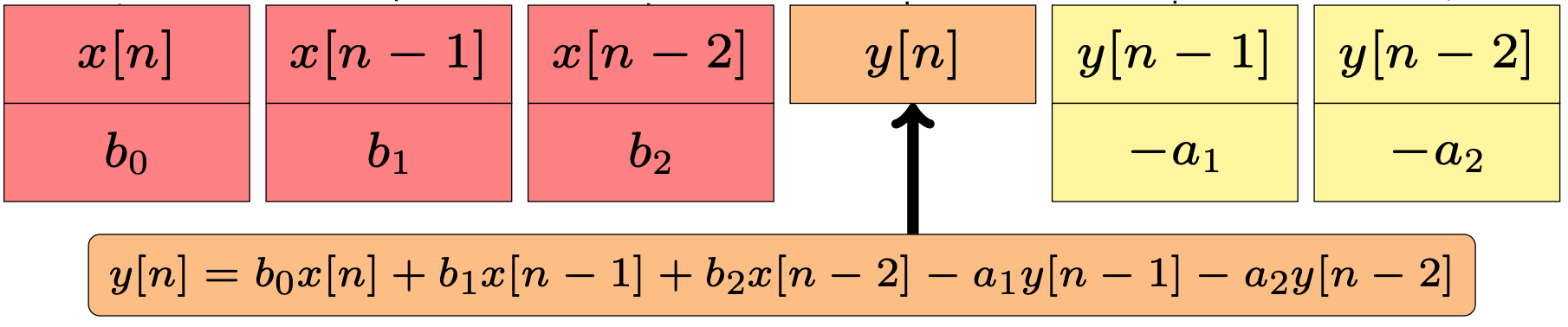
When a new input sample $x[n]$$x[n]$ is received, the input and output buffers are shifted to the right. The new input sample $x[n]$$x[n]$ is placed in the input buffer. The buffers and corresponding coefficient arrays are multiplied and added together. The result $y[n]$$y[n]$ is placed into the output buffer. Note that over time the input $x[n]$$x[n]$ and output $y[n]$$y[n]$ samples shift across these two arrays in the same way that the input $x[n]$$x[n]$ shifted across the input array in the FIR filter case.

The Matlab code below illustrates how to allocate and initialize a pair of buffers: one for input history and one for output history.

function y = myIIRfilter(b,a,x)
persistent zx zy; % Persistent internal filter memory
if isempty(zx)
    zx = zeros(size(b)); % Initialize input buffer to zero
    zy = zeros(size(a)); % Initialize output buffer zero
end

% Inputs
% b = [b[0], b[1], ..., b[M-1]] array of feed forward coefficients
% a = [a[0], a[1], ..., a[N-1]] array of feedback coefficients
% x = x[n] = the current input sample

% Outputs
% y = y[n] = the current output sample

% Shift data in buffer and write in the new input sample
... % Right shift buffers
... % Put new input sample into the input buffer

% Compute the filter output
y = ... % Point-by-point multiply and accumulate

... % Put new output sample into the output buffer

Your assignment is to finish writing the myIIRfilter function. Do not use built-in functions or vector operations.Use for loops where needed.

FIR Filter Design

FIR and IIR filter design are extensive topics in their own right. In this assignment, we will use a simple recipe to design FIR filters.

FIR Low Pass Filter

The following procedure designs the impulse response for a low-pass filter operating at a sample rate of $F_s$$F_s$ samples/second.

• The first step is to select the passband and stop band edge frequencies $F_{\text{pass}}$$F_\text{pass}$, and $F_{\text{stop}}$$F_\text{stop}$ in units of Hertz.
• Convert these to normalized frequencies $f_{\text{pass}}=F_{\text{pass}}/F_s$$f_\text{pass} = F_\text{pass} / F_s$ and $f_{\text{stop}}=F_{\text{stop}}/Fs$$f_\text{stop} = F_\text{stop} / Fs$.
• Compute $f_1=(f_{\text{stop}}+f_{\text{pass}})/2$$f_1 = (f_\text{stop} + f_\text{pass})/2$ and $f_2=(f_{\text{stop}}-f_{\text{pass}})/2$$f_2 = (f_\text{stop} - f_\text{pass})/2$.
• Select a filter order $N$$N$ which must be an odd integer, and compute $L=(N-1)/2$$L = (N-1)/2$.
• Compute the filter impulse response $h[n]$$h[n]$ using the Matlab code below. The impulse response has the form of a product of two sinc functions.

% Filter Specification
Fs = 8000; % samples/second
% Cut off frequencies
Fpass = 1000; % Hz
Fstop = 1500; % Hz
% Filter order
N = 101; % Length of filter impulse response (odd integer)

% FIR Filter Design Procedure
fpass = Fpass/Fs;
fstop = Fstop/Fs;
f1 = (fstop + fpass)/2;
f2 = (fstop - fpass)/2;
L = (N-1)/2;
n = [-L:L];
h = (sin(2*pi*f1*n) .* sin(2*pi*f2*n)) ./ ((pi*n) .* (2*pi*f2*n));
h(L+1) = 2*f1;

% Plot magnitude response
[H,F] = freqz(h,1,2^14,Fs); % Compute frequency response
subplot(211);
plot(F,abs(H),'LineWidth',2); % Plot magnitude response [linear]
xlabel('Frequency [Hertz]');
ylabel('Magnitude [linear]');
xlim([0 Fs/2]);
grid on;
subplot(212);
plot(F,20*log10(abs(H)),'LineWidth',2); % Plot magnitude response [dB]
xlabel('Frequency [Hertz]');
ylabel('Magnitude [dB]');
ylim([-80 5]); xlim([0 Fs/2]);
grid on; shg;

This script uses the freqz Matlab function to compute the frequency response of the FIR filter. This filter has a trapazoidal-shaped magnitude response as can be seen in the linear magnitude response plots below. It is flat in the pass band $[0,1000]$$[0, 1000]$ Hertz and rolls off linearly between the pass and stop band edge frequencies $[1000,1500]$$[1000, 1500]$ Hertz. No FIR filter has infinite attenuation in its stop band. This is a pretty good filter having 45 dB of attenuation at the stop band edge and rolling off to more than 70 dB of attenuation at 4000 Hz.

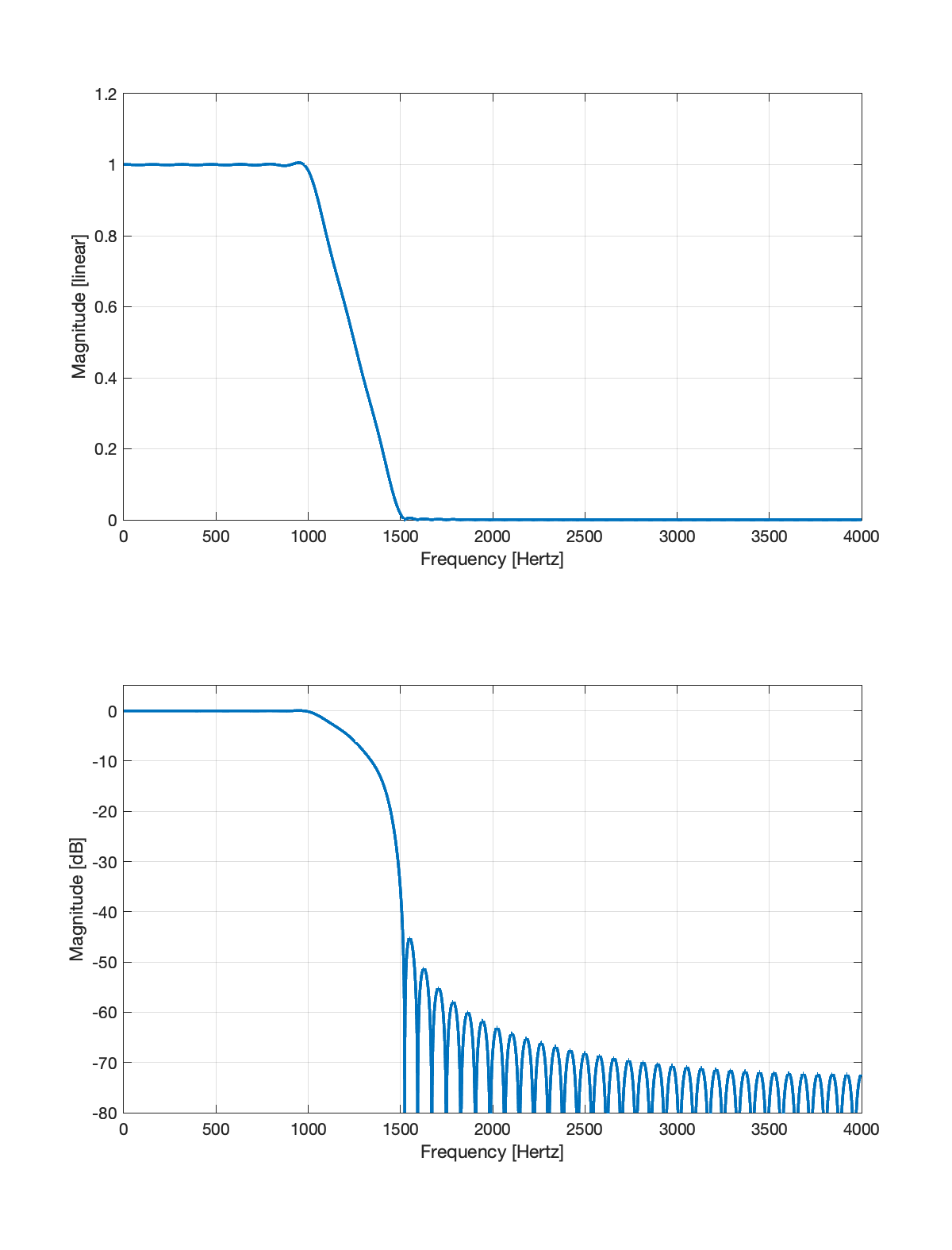
The impluse response (shown below) has a sinc-like shape.

You can modify this filter design script by changing the pass and stop band edge frequencies and by changing the filter order $N$$N$ which should be an odd integer.

FIR Bandpass Filter

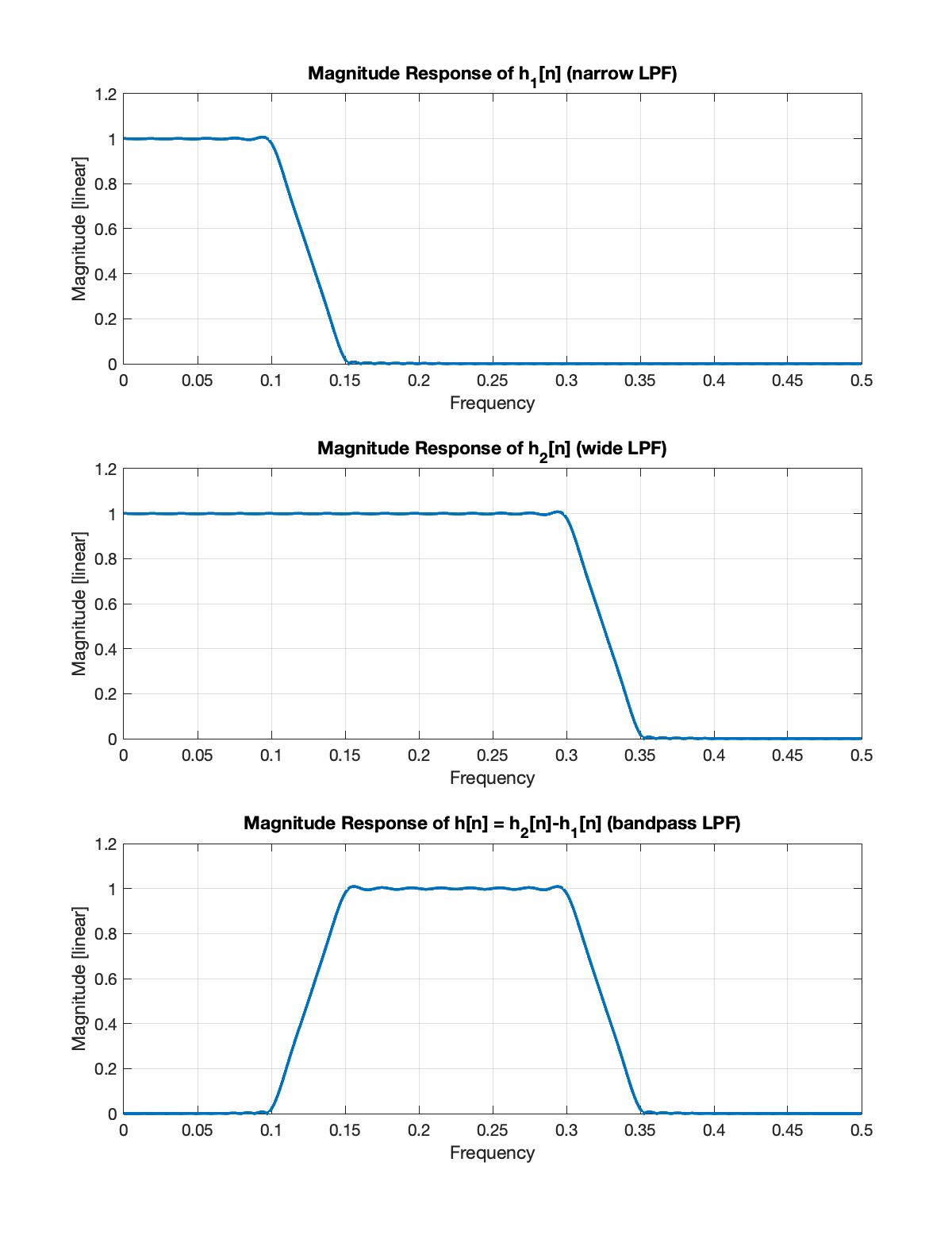
Consider two low pass filters designed to have the trapazoidal response above. Suppose the two filters have the frequencies characteristics shown in the table below.

Let $h_1[n]$$h_1[n]$ and $h_2[n]$$h_2[n]$ be the impulse responses of these filters and consider the FIR filter having impulse response

The magnitude responses of $h_1[n],h_2[n],h[n]$$h_1[n], h_2[n], h[n]$ are shown in the figure below. Can you see that the result of subtracting a narrow LPF from a wide LPF results in a bandpass filter (BPF)?

FIR High Pass Filter

The filter with impulse response $h_{\text{all}}[n]=\delta [n]$$h_\text{all}[n] = \delta[n]$ is an all pass filter because

The output is equal to the input. This filter passes everything!

We can combine an all pass filter $h_{\text{all}}[n]$$h_\text{all}[n]$ and a low pass filter $h_{\text{lpf}}[n]$$h_\text{lpf}[n]$ to build a high pass filter like this

To make this work, the delta function has to "line up" with the sinc function main lobe in the low pass filter. We'll see why this is the case later on in the course. For now, consider the Matlab code below to make this work.

L = 50; N = 2*L+1; % Odd integer
n = [-L:L];
% Design LPF
f1 = 0.125; f2 = 0.025;
hlpf = (sin(2*pi*f1*n) .* sin(2*pi*f2*n)) ./ ((pi*n) .* (2*pi*f2*n));
hlpf(L+1) = 2*f1;
% Design all pass filter
hall = zeros(size(hlpf));
hall(L+1) = 1; % This is the "delta"
% Design HPF
hhpf = hall - hlpf;
% Compute frequency response
[Hhpf,F] = freqz(hhpf,1,2^14,1);

% Visualization
figure();
subplot(211);
stem(n+L,hlpf,'LineWidth',2);
xlabel('Index');
ylabel('Amplitude');
title('LPF Impulse Response')
grid on;
subplot(212);
stem(n+L,hall,'LineWidth',2);
xlabel('Index');
ylabel('Amplitude');
title('All Pass Impulse Response (delta function)')
grid on;

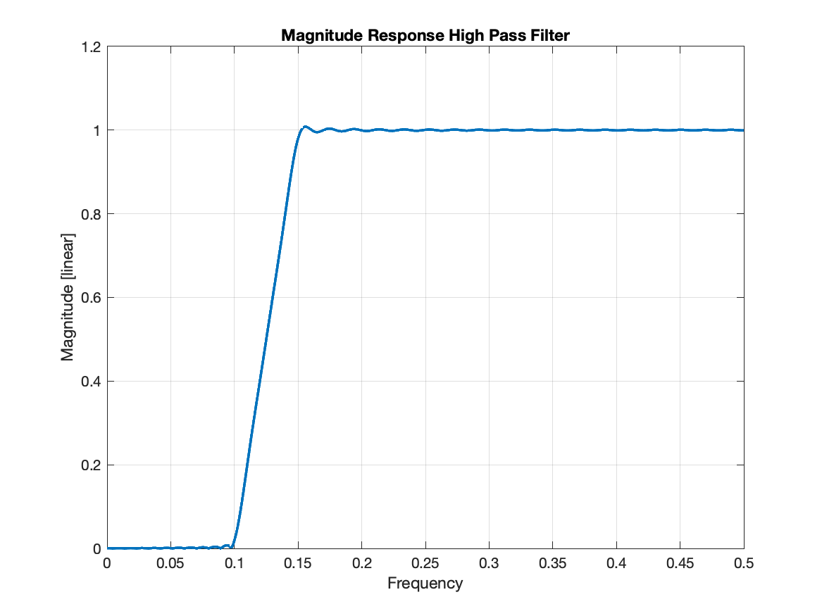
figure();
plot(F,abs(Hhpf),'LineWidth',2);
xlabel('Frequency');
ylabel('Magnitude [linear]');
title('Magnitude Response of High Pass Filter');
grid on;
shg;

Here is a plot of the impulse responses of the low pass and all pass filters. Can you see that the delta in the all pass filter "lines up" with the main lobe of the low pass filter impulse response?

Here is a plot of the high pass filter magnitude response. Can you see that it stops low frequencies and passes high frequencies? Hence the name high-pass filter.

Given the principles described here, how would you design a band-stop filter?

IIR Filter Design

Matlab has several built-in IIR filter design procedures. We will learn about these later in the course. In this lab assignment, several IIR filter designs will be given.

IIR Shelving Filter

The web page Shelving Filter gives the difference equation for a low-shelf shelving filter with $N=M=2$$N=M=2$.

IIR Notch Filter

A notch filter may be designed as follows for processing data sampled at rate $F_s$$F_s$.

• Compute $q=\exp (-20\pi /F_s)$$q = \exp(-20\pi/F_s)$.
• Choose a notch frequency $F_n$$F_n$.
• Compute a normalized notch frequency $f_n=F_n/F_s$$f_n = F_n/F_s$ and ${\omega }_n=2\pi f_n$$\omega_n = 2\pi f_n$.
• Compute the filter coefficients $b[n]$$b[n]$ and $a[n]$$a[n]$ using the Matlab code shown below.

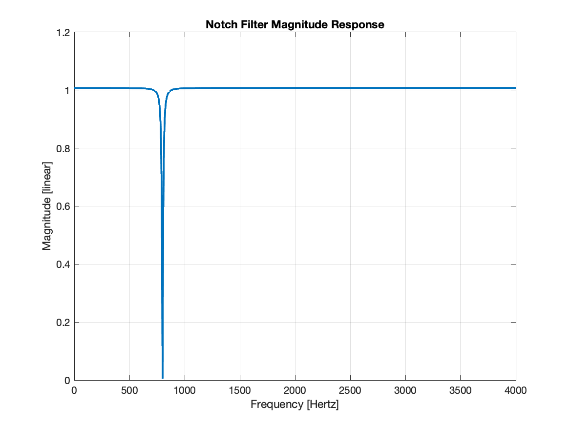
b = [1, -2*cos(omega_n), 1]; a = [1, -2*q*cos(omega_n), q^2];

The notch filter has the magnitude response shown below. It was designed to have a notch at 800 Hz and a sample rate of 8000 Hz. The reason for calling this a notch filter is clear from the magnitude response. It has unity gain across all frequencies except for those frequencies near the notch frequency where it has a gain of zero. If this filter was applied to a song with a note at 800 Hz, this filter would remove those notes completely.

Other IIR Filter Types

IIR filters have a wide variety of applications. IIR filters can be designed to exhibit excellent frequency response characteristics. Designing other types IIR filters will be considered later in the course.

Assignment

FIR Filtering

1. Complete the FIR filtering function and turn in a printout of your code. Do not use built-in functions or vector operations. Use for loops where needed. Write the filtering function using a single for loop.

2. Let the impulse response be $\mathbf{h}=[1,2,3,4,4,3,2,1]$$\mathbf{h} = [1, 2, 3, 4, 4, 3, 2, 1]$ and prove that the code is correct by inputting an impulse sequence $[1,0,0,0,0,\cdots ,0]$$[1, 0, 0, 0, 0, \cdots, 0]$ and verifying that the output is the impulse response $h[n]$$h[n]$. You will need to write a script that calls your filtering code for each sample in the impulse sequence.

3. Let the impulse response be $\mathbf{h}=[0.0625,0.2764,0.4182,0.2764,0.0625]$$\mathbf{h} = [0.0625, 0.2764, 0.4182, 0.2764, 0.0625]$ and the input be $x[n]=\cos (2\pi 0.422n)$$x[n] = \cos(2\pi 0.422 n)$.

   a. Compute the filter output $y[n]$$y[n]$ for $n=0,1,2,\cdots ,20$$n=0, 1, 2, \cdots, 20$ and show that after an initial transient the steady state value of the output is zero.

   b. Using the freqz function, plot the magnitude response assuming the sample rate is $F_s=1$$F_s = 1$ sample/second.

   c. Using the magnitude response, explain why the steady state output is zero.

4. Design a band-stop filter by combining all-pass and low-pass filters.

   a. Show how to compute the impulse response.

   b. Make a plot of the filter magnitude response.

IIR Filtering

4. Complete the IIR filtering function and turn in a printout of your code. Do not use built-in functions or vector operations. Use for loops where needed. Write the filtering function using a single for loop for the feed forward section and a single for loop for the feedback section.

5. Use the filter coefficients for the shelving filter and process the signal on the shelving filter web page. Use the original audio as the input signal rather than the whole song.

   a. Make spectrogram plots of the input and output to illustrate that the shelving filter performs as expected.

   b. Using the freqz function, plot the filter magnitude response using the sample rate in the audio file.

   c. What audible effect does the shelving filter impart to the signal? How does the magnitude response of the shelving filter predict this result?

6. Design a notch filter to cut out the note Bb4=A#4 which has a frequency of 466.16 Hz (https://pages.mtu.edu/~suits/notefreqs.html). This note occurs multiple times in the introduction to the song "Fireflies" by Owl City. Here is an audio clip. To design the notch filter, you will need the audio sample rate and that can be obtained from the audio file using the Matlab command shown below. Process the audio clip using your IIR filtering code and make spectrogram plots of the input signal $x[n]$$x[n]$ and the output signal $y[n]$$y[n]$. Can you see that the notch filter removed the notes at 466.16 Hz?

[x,Fs]=audioread('fireflyintro.wav'); % Fs = 44,100 samples/second