Chapter 2: Multi-Armed Bandits
Jake Gunther
2019/13/12
Evaluative vs. Instructive Learning
Pure Evaluation
Tells how good an action was
Depends entirely on the action taken
Pure Instruction
Tells what action to take
Independent of action taken
This is supervised learning
Associative vs. Nonassociative Settings
Associative Setting
Choosing different actions in different settings
Nonassociative Setting
Learning to act in only one situation
Context for Chapter 2
We are going to study evaluative RL in nonassociative setting.
\(K\)-armed bandits
What is a \(K\)-Armed Bandit?
for i=1, 2, ..., N
   (1) choose action in {A_1, A_2, ..., A_k}
(2) draw reward from PDF(action)- Repeatedly choose from \(k\) actions according to some policy
- Receive reward drawn from pdf depending on action
- Objective: maximize the total expected reward over \(N\) actions
- What policy does this?
- What are good/bad policies?
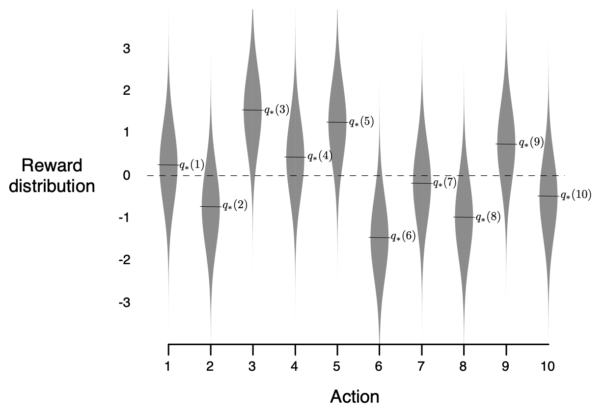
Example: Slot Machine

Pull the best arm (action).
The reward is random (governed by a PDF).
Each arm (action) has different reward PDF.
Some Math
Definitions
- \(A_t =\) action selected at time \(t\)
- \(R_t =\) reward for action \(A_t\) at time \(t\)
- \(q_\ast(a) = E[R_t | A_t = a] =\) value of action \(a\)
- \(Q_t(a)\) is an estimate of \(q_\ast(a)\)
- \(\text{Policy}: Q_t \mapsto A_t\) (maps value to action)
Indicator Function
\[ 1_\text{predicate} = \begin{cases} 1, & \text{predicate is true} \\ 0, & \text{predicate is false} \end{cases} \]
\[ 1_{A_i = a} = \begin{cases} 1, & A_i = a \\ 0, & A_i \neq a \end{cases} \]
- If \(\text{predicate}\) involves an RV, then \(1_\text{predicate}\) is an RV, i.e. function of an RV.
Value Estimates
Sample Average Estimate
\[ \begin{align} q_\ast(a) &= E[R_t | A_t = a] \\[1em] Q_t(a) &= \frac{\displaystyle \sum_{i=1}^{t-1} R_i 1_{A_i=a}} {\displaystyle \sum_{i=1}^{t-1} 1_{A_i=a}} \end{align} \]
Convergence:
\(Q_t(a) \rightarrow q_\ast(a)\)
as \(\displaystyle \sum_{i=1}^{t-1} 1_{A_i=a} \rightarrow \infty\)
Convergence speed?
Policies
Policy if \(q_\ast(a)\) is known?
How would you exploit knowlege of the value function \(q_\ast(a) = E[R_t |A_t=a]\) to maximize total expected rewards in \(N\) trials?
Wouldn’t you always choose the maximum? \[ A_t = \arg \underset{a}{\max} Q_t(a) \]
This is called a greedy policy
Policy if \(q_\ast(a)\) is unknown?
- If \(q_\ast(a)\) is unknown, then use the estiamte \(Q_t(a)\).
Greedy Policy
\[ A_t = \arg \underset{a}{\max} Q_t(a) \]
- Choose action with best estimated value
- Greed always chooses the best action
- If \(Q_t(a) = q_\ast(a)\), then greed is good (optimal)
- If \(Q_t(a) \neq q_\ast(a)\), then greed may be bad (sub-optimal)
Notation
- \(q_\ast(a)\) not a function of \(t\). Assumed to be constant.
- \(Q_t(a)\) is a function of \(t\). This function changes with time. This is learning.
- The greedy action \(A_t = \arg \underset{a}{\max} Q_t(a)\) may change with time too. This is learning.
Exploitation vs. Exploration
- Greedy action exploits knowledge of \(Q_t(a)\)
- Non-greedy actions explore other actions
- If \(Q_t(a) \neq q_\ast(a)\), then exploration can find super-greedy actions that can be used to improve the estimate \(Q_t(a)\).
Short Run vs. Long Run
Short run (few time steps available)
- Exploitation is probably best in the short run
- Greedy actions maximize immediate rewards
Long run (many time steps available)
- Exploration can find better/best actions which can be exploited many times in the long run
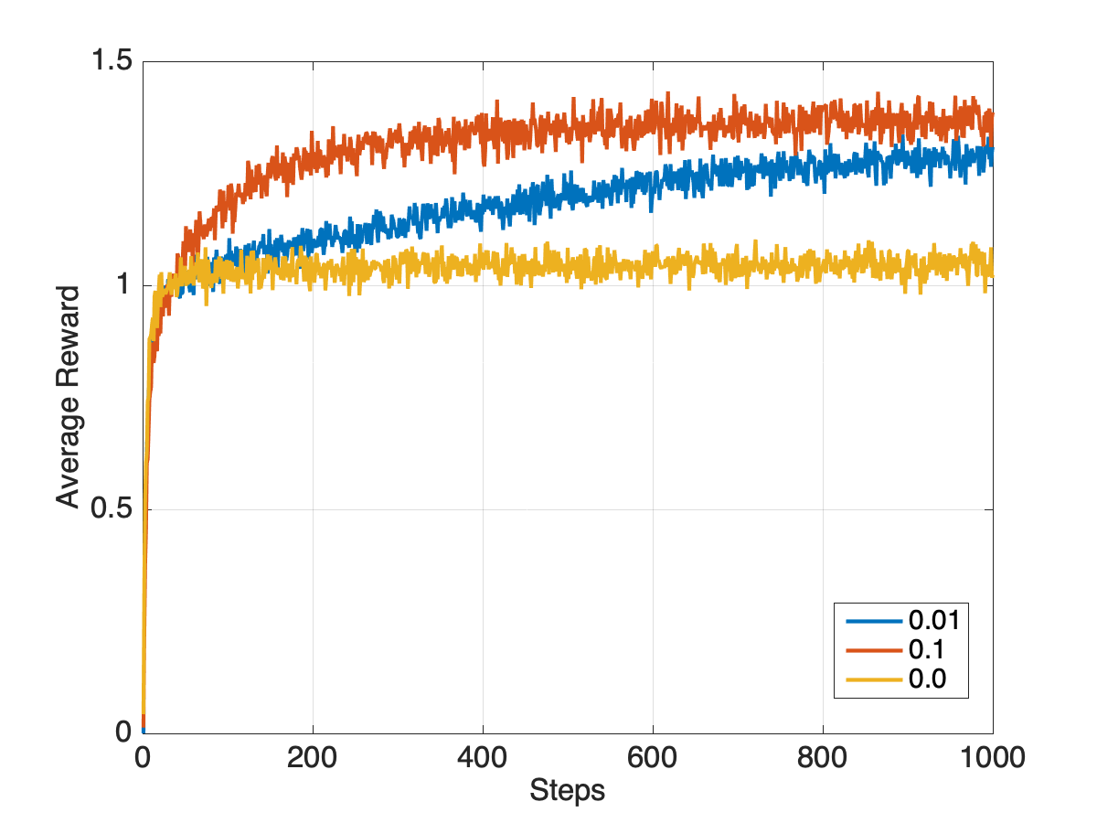
\(\varepsilon\)-Greedy Policy
\[ A_t = \begin{cases} \arg \underset{a}{\max} Q_t(a), & \text{with prob} \;1-\varepsilon \\ a_i, \;i \sim U[1, 2, \cdots, k], & \text{with prob} \;\varepsilon \end{cases} \]
- Greedy most of the time (exploitation)
- Randomly explore non-greedy actions
Learning Algorithm
Learning
- Learning means updating the value estimate \(Q_t(a)\)
- Selected actions evolve as \(Q_t(a)\) changes
- Learning algorithms explore and exploit (need both, how much of each?)
- Greedy policy is non-learning (it does adapt/evolve, however)
- \(\varepsilon\)-Greedy policy learns
Learning vs. Optimization
Parameter Optimization
\[ \hat{x} = \arg \max_x f(x) \]
- Choose parameter \(x\) to maximize an objective function \(f\)
Learning
- Objective: maximize total expected reward
- Policy: \(Q_t \mapsto A_t\) (take action)
- Bandit: \(A_t \mapsto R_t\) (receive reward)
- Update: \(Q_t \mapsto Q_{t+1}\) (update estimate)
- Note: \(Q_t \underset{t\rightarrow \infty}{\longrightarrow} q_\ast\) is sufficient (what algorithms?)
- Learning is different from parameter optimization
Learning
- Move from what we know now (at time \(t\)) through interaction with the environment to new knowledge (at time \(t+1\))
\[ \underset{\begin{array}{c}\text{old} \\ \text{knowledge}\end{array}}{Q_t}\overset{\begin{array}{c}\text{policy:} \\ \text{exploit} \\ \text{explore} \end{array}}{\longrightarrow} \underset{\text{action}}{A_t} \overset{\begin{array}{c} \text{bandit or} \\ \text{environment}\end{array}}{\longrightarrow} \underset{\text{action}}{R_t} \overset{\begin{array}{c} \text{learning} \\ \text{update} \end{array}}{\longrightarrow} \underset{\begin{array}{c}\text{new} \\ \text{knowledge}\end{array}}{Q_{t+1}} \]
Reinforcement Learning
Putting it all Together
- Action space defined
- Reward function
- pdf known
- simulation
- real world
- Value Estimator
- initialization
- update
- Policy (maps value estimator to actions)
Put these together and you have an algorithm for RL
Testbed
Performance
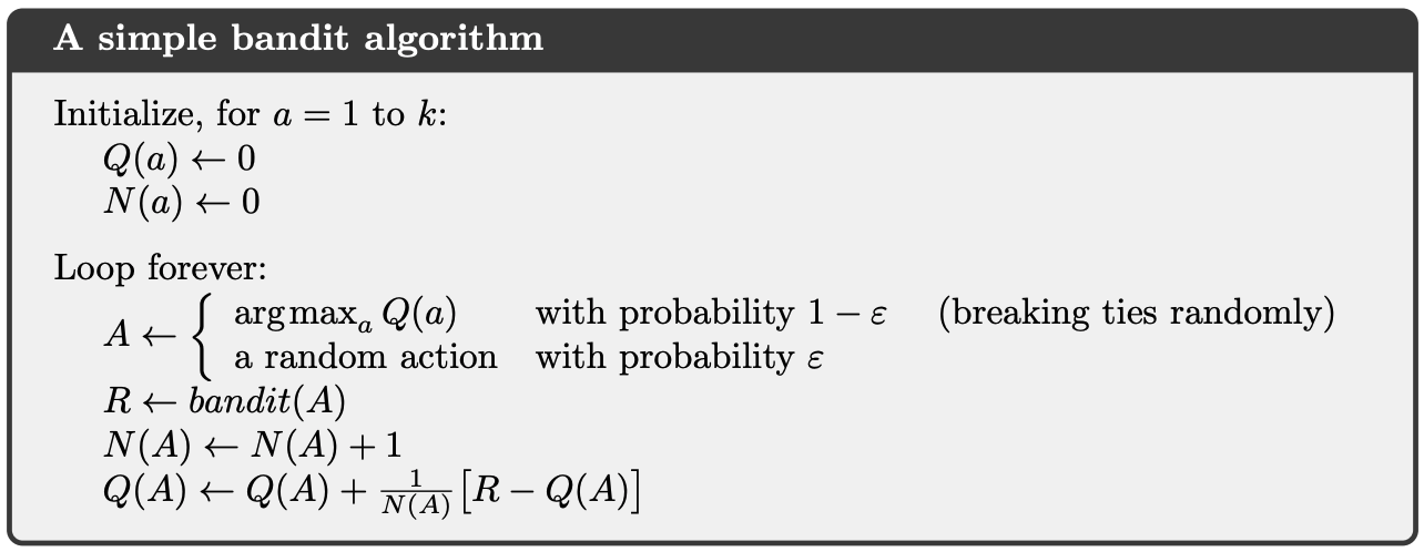
Incremental Implementation
Calculation Trick
\[ Q_n = \frac{R_1 + R_2 + \cdots + R_{n-1}}{n-1} \]
- \(R_n=\) reward after a particular action
- \(Q_n=\) value estimate for particular action
\[ \begin{align} Q_{n+1} &= \frac{1}{n} \sum_{i=1}^n R_i = \frac{1}{n} \left( R_n + \sum_{i=1}^{n-1} R_i \right) \\ &= \frac{1}{n} \left( R_n + \frac{n-1}{n-1}\sum_{i=1}^{n-1} R_i \right) \\ &= \frac{1}{n} \left( R_n + (n-1) Q_n \right) \\ &= \frac{1}{n} \left( R_n + n Q_n - Q_n\right) \\ &= Q_n + \frac{1}{n} \left[ R_n - Q_n \right] \end{align} \]
Update Formula
\[ \text{NewEst} \leftarrow \text{OldEst} + \text{StepSize}\left[\text{Target} - \text{OldEst}\right] \]
\[ Q_{n+1} = Q_n + \frac{1}{n} \left[ R_n - Q_n \right] \]
- \(\left[\text{Target} - \text{OldEst}\right]\) is the error in the estimate
- Step is in a direction that reduces the error on average
- The target is an RV
- StepSize is time varying, denoted by \(\alpha_n(a)\)
Simple Bandit Algorithm
Nonstationary Problems
Stationary
- Reward PDF invariant
- \(\alpha_n(a) = \frac{1}{n}\) allows convergence to a stationary reward PDF
- Puts less and less weight on recent errors
- Fails in nonstationary case
Nonstationary
- Reward PDF changes
- Real problems nonstationary
- Want more weight on recent errors
- \(\alpha_n(a) = \alpha\) continuous adaptation
- Uncertainty \(\Rightarrow\) always explore
Constant Step Size
\[ \begin{align} Q_{n+1} &= Q_n +\alpha\left[ R_n - Q_n\right] = \cdots \\ &=(1-\alpha)^n Q_1 + \sum_{i=1}^n \alpha(1-\alpha)^{n-i} R_i \end{align} \]
- Exponential recency-weighted average
- Eventually the initial condition is forgotten
- More weight given to recently observed rewards
Initial Values
Initial Values
- \(Q_n(a)\) is biased by initial values \(Q_1(a)\)
- Bias fades for \(\alpha_n(a)=\alpha\)
- Bias expires for \(\alpha_n(a)=\frac{1}{n}\) once \(a\) is chosen once
- Can set \(Q_1(a) = 0\) for all \(a\)
- \(Q_1(a)\) are user selectable parameters
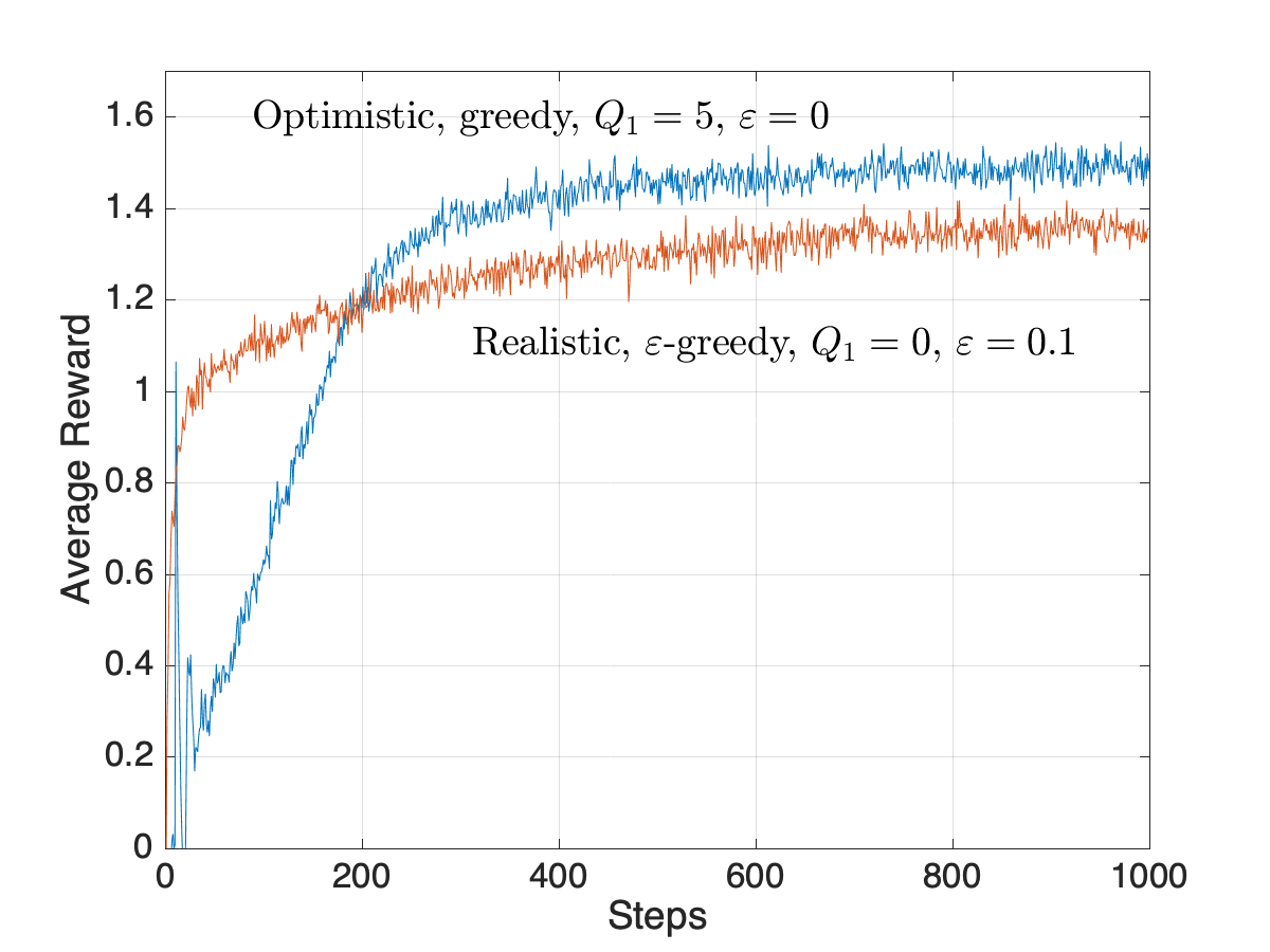
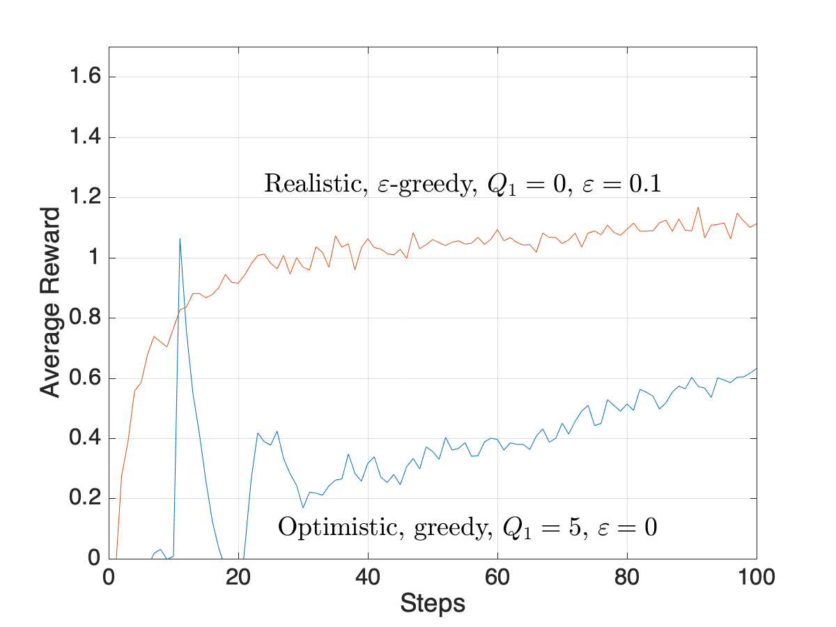
Optimistic Initial Values
- Setting \(Q_1(a)\) unreasonably high forces an effect like exploration, even for pure greedy policies
- Example: \(\alpha=0.1\) in recursive update for \(Q_n(a)\)
 { width=50% }
 { width=50% }
Observations
- Optimistic initial values is a trick to force early exploration
- It works well in stationary environments, but not nonstationary
- Sample average methods also treat beginning of time as special case
Preferences and Policy PDF
Definitions
- \(H_t(a) =\) relative preference for action \(a\)
- \(Pr\{A_t=a\} = \pi_t(a) = \frac{e^{H_t(a)}}{\sum_{b=1}^{k} e^{H_t(b)}} =\) policy PDF
- Actions selected at random from \(\pi_t(a)\)
- \(E[R_t] = E[ E[R_t |A_t] ] = E[q_\ast(A_t)]=\displaystyle \sum_a \pi_t(a) q_\ast(a)\)
Policy Gradient
- Homework: Show that gradient ascent leads to the updates below (see pg. 38+)
\[ H_{t+1}(a) = H_t(a) + \alpha \frac{\partial E[R_t]}{\partial H_t(a)} \quad \text{(gradient ascent)} \]
\[ \begin{align} H_{t+1}(A_t) &= H_t(A_t) + \alpha (R_t - \bar{R}_t)(1-\pi_t(A_t)) \\ H_{t+1}(a) &= H_t(a) - \alpha (R_t - \bar{R}_t)\pi_t(A_t), \quad a \neq A_t \end{align} \]