Convolution Lab

Resources

Video

Slides

Introduction

In this assignment, you will write a custom 1-D convolution function in Matlab and use it to pass signals through LTI systems by convolution with the system impulse response. Matlab has a built-in convolution function called conv. Later on you can use conv, but right now while you're learning about the mechanics of convolution, you must write your own.

Definition of Convolution

The mathematical definition of convolution is given by

The general convolution definition in ($\text{1}$$\ref{eq:conv}$) accommodates infinite length inputs $x[n]$$x[n]$ and impulse responses $h[n]$$h[n]$. In this assignment, we will focus on the finite case where the input $x[n]$$x[n]$ has length $N$$N$ and the impulse response $h[n]$$h[n]$ has length $L$$L$. We also assume that both $x[n]$$x[n]$ and $h[n]$$h[n]$ "start" at time $n=0$$n=0$. Given these specifications, the convolution sum may be written as

Finite length $x[n]$$x[n]$ and $h[n]$$h[n]$ affect the convolution sum in two ways.

1. Convolution of length-$N$$N$ and length-$L$$L$ sequences produces a output sequence $y[n]$$y[n]$ of length $N+L-1$$N+L-1$. Therefore, output $y[n]$$y[n]$ is defined for $n=0,1,2,\cdots ,N+L-2$$n=0, 1, 2, \cdots, N+L-2$.

2. The sequences $x[n]$$x[n]$ and $h[n]$$h[n]$ are assumed to be zero outside their support sets:

Removing from the convolution sum terms that are zero due to these limits leads to the messy looking limits on the summation.

Mechanics of Convolution

The mathematical definitions of convolution in ($\text{1}$$\ref{eq:conv}$) and ($\text{2}$$\ref{eq:convfin}$) present convolution as a sequence of operations. To compute the output $y[n]$$y[n]$ at time $n$$n$, do the following:

1. Time reverse the impulse response and shift it to time $n$$n$. At this point the output time $n$$n$ is fixed. Think of $h[n-k]$$h[n-k]$ as being a function of $k$$k$.

2. Multiply $x[k]h[n-k]$$x[k]h[n-k]$ for a suitable range of $k$$k$ values.

3. Sum the products and assign the result to $y[n]=\sum _{k}x[k]h[n-k]$$y[n] = \sum_k x[k] h[n-k]$.

By repeating these steps for each value of $n$$n$, the output sequence $y[n]$$y[n]$ is computed. This process requires two for loops: an outer loop over the output times $n$$n$ and an inner loop over $k$$k$ to form and sum the products.

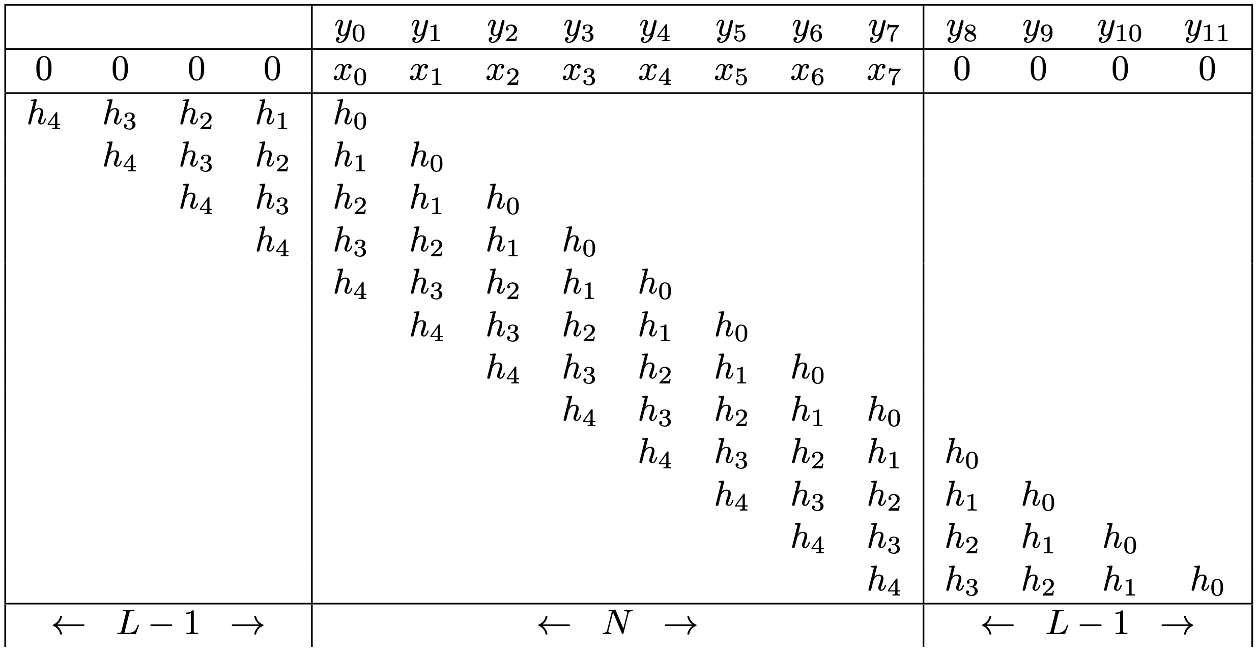
There are multiple ways to implement convolution in code. The approach we will follow takes inspiration from the table depicted above. In this example $N=8$$N=8$ and $L=5$$L=5$. The length of the output $y[n]$$y[n]$ is $N+L-1=12$$N+L-1 = 12$. These twelve values are laid out in the first row of the table. The table uses the compressed notation of subscripts $y_n$$y_n$ to represent $y[n]$$y[n]$. The second row of the table lays out the eight values of the input sequence $x_n$$x_n$. The other rows of the table show time-reversed shifts of the impulse response $h_{n-k}=h[n-k]$$h_{n-k} = h[n-k]$ for twelve shifts $n=0,1,2,\cdots ,11$$n=0, 1, 2, \cdots, 11$, one shift for each output value. Note that whereas the input $x_n$$x_n$ and output $y_n$$y_n$ appear in natural order with the subscript/index increasing from left to right, the impulse response is laid out in time-reversed order with the subscript/index decreasing from left to right.

To compute the output $y_n$$y_n$ at time $n$$n$, multiply the sequence $h_{n-k}$$h_{n-k}$ on the $n^{\text{th}}$$n^\text{th}$ row of the table by the input sequence $x_n$$x_n$ on the second row of the table, sum the products, and assign the result to the appropriate value $y_n$$y_n$ in the top row of the table. A design decision that greatly simplifies the code is to pad the input sequence $x_n$$x_n$ with $L-1=4$$L-1=4$ zeros on both sides. Zero-padding eliminates the need to encode the complicated limits in the finite summation in ($\text{2}$$\ref{eq:convfin}$). Zero-padding is justified due to the assumption in equation in ($\text{3}$$\ref{eq:xlen}$).

The matlab script below is a barebones script for testing out the ideas presented above. After creating a simple input signal and impulse response, the script calls the custom convolution function myconv. The rest of the script is plotting.

% Input signal
N = 8;
x = ones(N,1);

% Impulse response
L = 5;
h = ones(L,1);

% Convolve - call custom convolution function
y = myconv(x,h);

% Visualize
M = N+L-1; % Compute length of output
n = [0:M-1]; % Construct a time sequence
stem(n,y,'LineWidth',2); % Plot
xlabel('Time');
ylabel('Output Amplitude');
title('Output Sequence y[n]');
grid on;
shg; % Show handle graphics

The basic structure of the custom convolution function myconv appears below. This code is placed in a separate file called myconv.m. Your job is to figure out the array indexes in the inner convolution loop.

function y = myconv(x,h)
N = length(x); % Length of x[n]
L = length(h); % Length of h[n]

K = N+2*(L-1); % Length of zero-added x[n]
xzp = zeros(K,1); % Allocate memory
xzp(L:L+N-1) = x; % Zero-pad x[n]

M = N+L-1; % Length of output sequence
y = zeros(M,1); % Allocate memory
for n=1:M % Loop over output times
    for k=1:L % Multiply-accumulate loop
        y(n) = y(n) + xzp( ??? )*h( ??? ); % <= Array indexes?
    end
end

If done correctly, the result should look like this.

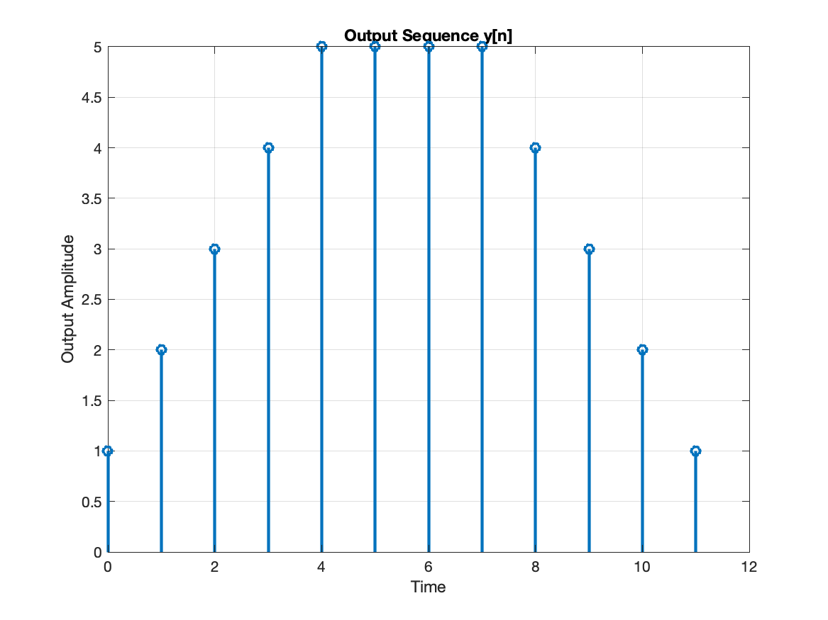
The output sequence is $[1,2,3,4,5,5,5,5,4,3,2,1]$$[1, 2, 3, 4, 5, 5, 5, 5, 4, 3, 2, 1]$.

To understand the Matlab code, you can set breakpoints and run the script in debug mode. You can examine variables and make plots to visualize signals at each point and in each step of a loop. Refer back to the table above and make your code implement the operations implied by the table.

Process Audio Signal with Low Pass Filter

Download the audio file and the impulse impulse response file. The script below illustrates how to load audio data from a WAV file and to read the impulse response from the binary file. It uses your myconv function to filter the input signal by convolution with the impulse response. It also plots the input and output signals in the time domain, the impulse response of the filter, the magnitude response of the filter, and spectrograms of the input and output signals. I am providing this script for educational purposes. There are over 80 lines of code in this script. Most of these lines are for visualization. This script illustrates how to:

1. Write commented and organized code in Matlab.

2. Make time domain plots that have (1) labeled axes, (2) title, (3) legend where appropriate, (4) a grid, (5) time axis with units of seconds, (6) plot two data sets in one axis.

3. Make frequency responsen plots that have (1) labeled axes, (2) title, (3) frequency axis with units of Hertz, (4) decibel scaled y-axis, (5) adjust axis limits.

4. Make spectrograms that have (1) labeled axes, (2) title, (3) color bar, (4) good intensity scaling, (5) several subplots in a figure.

Please study this code and learn how it works so that you can use Matlab, develop good coding habits, create beautiful visualizations of signals in time and frequency domains.

% Read in impulse response
fid = fopen('lpf_260_400_44100_80dB.bin','rb');
header = fread(fid,5,'int'); % Read in header
h = fread(fid,inf,'float'); % Read in impulse response
L = length(h);
fclose(fid);

% Read in input signal
[x,Fs] = audioread('fireflyintro.wav');
N = length(x);

% Convolve using custom convolution function
y = myconv(x,h);
M = N+L-1;

% Write out the audio signal
audiowrite('fireflyintro_output.wav',y,Fs);

% Visualize the filter impulse response
figure();
plot([0:L-1],h,'LineWidth',2);
xlabel('Sample Index');
ylabel('Amplitude');
title('Impulse Response');
grid on;
shg;
print -dpng impulse_response.png

% Visualize the filter frequency response
NFFT = 2^14;
F = Fs * ([0:NFFT-1]/NFFT - 0.5); % Frequency vector [Hertz]
H = fftshift(fft(h,NFFT)); % Compute Fourier transform
figure();
plot(F,20*log10(abs(H)),'LineWidth',2); % Plot magnitude response in dB
axis([0, 1200, -100, 10]); % Set axis limits
xlabel('Frequency [Hertz]');
ylabel('Magnitude [dB]');
title('Frequency Response');
grid on;
shg;
print -dpng magnitude_response.png

% Visualize signals in time domain
figure();
t = [0:N-1]/Fs; % Time vector [seconds]
plot(t,x); hold on;
t = [0:M-1]/Fs; % Time vector [seconds]
plot(t,y); hold off;
xlabel('Time [seconds]');
ylabel('Amplitude');
legend('Input x[n]','Output y[n]');
title('Input & Output Signals');
grid on;
shg;
print -dpng audio_timedomain.png

% Plot spectrograms of input and output signals
figure();
subplot(211);
[S,F,T] = spectrogram(x,hamming(NFFT),round(0.9*NFFT),NFFT,Fs);
imagesc(T,F,20*log10(abs(S)),[0 50]);
colorbar;
set(gca,'YDir','normal');
ylim([0 1500]);
xlabel('Time [seconds]');
ylabel('Frequency [Hertz]');
title('Spectrogram of the Input x[n]');
grid on;

subplot(212);
[S,F,T] = spectrogram(y,hamming(NFFT),round(0.9*NFFT),NFFT,Fs);
imagesc(T,F,20*log10(abs(S)),[0 50]);
colorbar;
set(gca,'YDir','normal');
ylim([0 1500]);
xlabel('Time [seconds]');
ylabel('Frequency [Hertz]');
title('Spectrogram of the Output y[n]');
grid on;
shg;
orient tall;
print -dpng audio_spectrograms.png

Pictures of the various signals and responses are included here.

Note that the impulse response has a sinc-like shape.

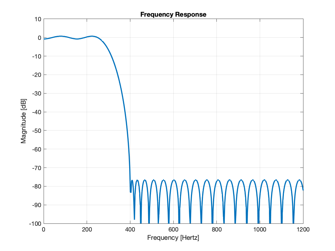
This filter is called a low-pass filter because it passes low frequency components (approximately 0 dB attenuation) and attenuates higher frequencies by about 80 dB. Notice a small amount of "ripple" in the passband response and the uniform ripple amplitude in the stop band. Note that the frequency response extends to higher frequencies. This plot is zoomed in to show the lower 1,200 Hz.

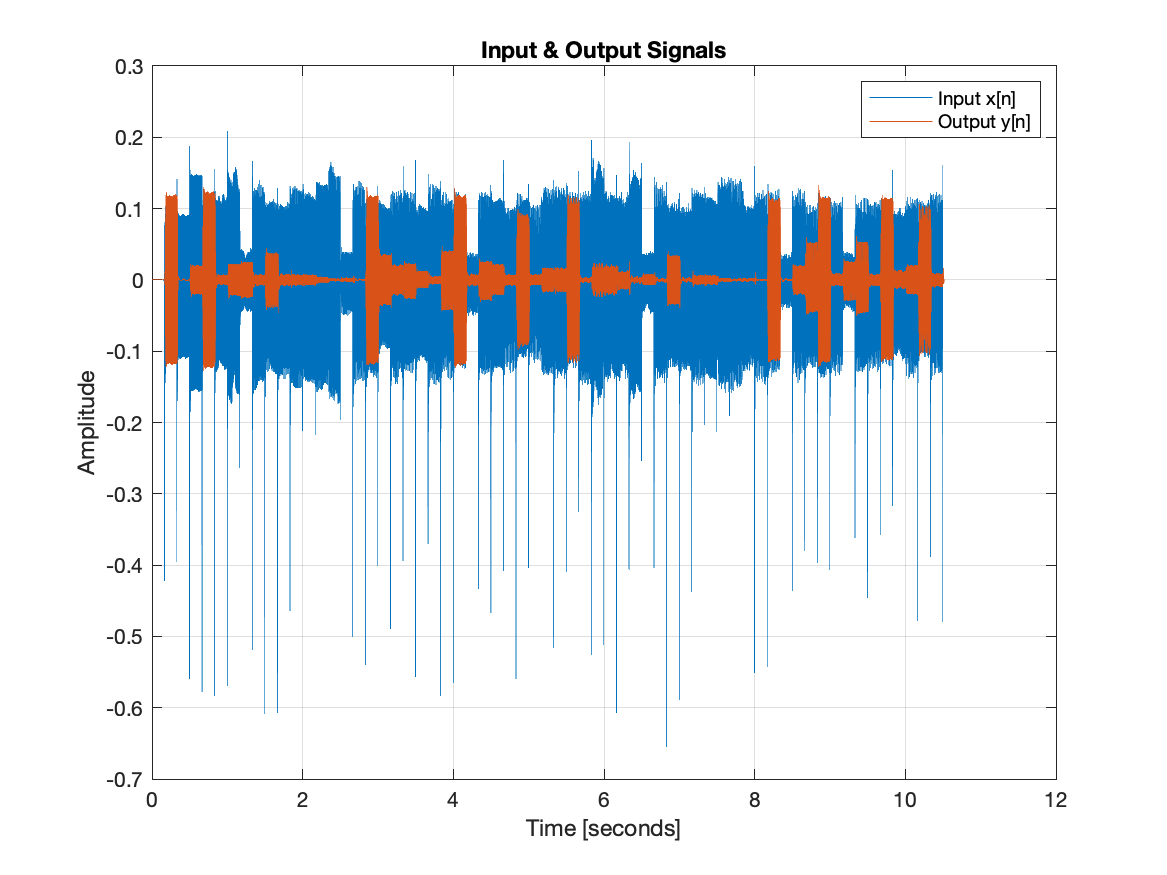
Can you see that the filter rejected some of the notes in this song?

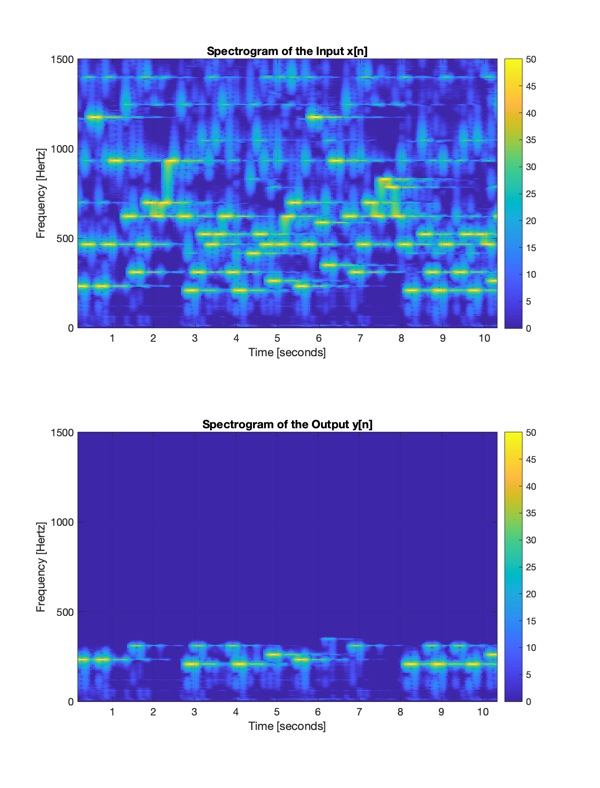
These spectrograms show how energy in the input and output signals is distributed over time and frequency. The spectrogram of the input shows that it contains energy at frequencies above 400 Hz, but these components have been removed in the output spectrogram. The spectrograms explicitly show that the filter rejects high frequencies. Can you hear the effect when you listen to the input and output signals?

Assignment

Write a report that addresses the following questions. This report includes Matlab plots. When making plots in Matlab or by hand, please keep the following points in mind.

• Label the axes. (xlabel, ylabel)

• Include a title. (title)

• If there are multiple lines on a plot, include a legend. (legend)

• The lines on plots should be visible (thick enough). (plot(...,'Linewidth',2))

• Intensity images should include a colorbar. (colorbar)

• Set the axis ranges to visualize the desired features of the function or image being plotted. (xlim, ylim, axis)

Here are the report questions (five points for each question).

1. What are the array indexes you used for xzp(...) and h(...) in the myconv code?

2. Include a stem plot showing the convolution of the following sequences: x = [1, 2, 3, 4, 5, 6, 7, 8] and h = [1 2 3 4]. Also list the values $y[n]=x[n]\ast h[n]$$y[n] = x[n] \ast h[n]$ in the convolution result.

3. Plot the impulse response of the filter used in the audio example.

4. Plot the dB-magnitude response of the filter used in the audio example.

5. Use the magnitude response plot to explain why the filter in the audio example is considered to be a low-pass filter. Describe the features of the passband and the stop band of this filter. What frequencies does this filter "pass" and what frequencies does this filter "stop"?

6. What would the response of a high pass filter look like? Make a sketch.

7. Plot spectrograms of the audio signals at the filter input and output (2 spectrogram plots).

8. Use the spectrograms to describe the action of this filter on a signal.

9. Plot the filter input and output signals on the same axis (time-domain plot).

10. There are times when the input signal is large and the output signal is essentially zero. See for example the intervals 2-3 seconds and 7-8 seconds in the time-domain plot. Use the filter magnitude response and the spectrograms to explain what is happening in these intervals. Why is the output signal zero there?

11. Attach your Matlab code.

Policy note: Please include your answers to these questions, the plots, and your code in a single PDF file uploaded to Canvas.