Background

• Large number of states
• Tabulating value function intractable
• Use function approximation
• \(\hat{v}(s,\mathbf{w}) \approx v_\pi(s)\)
• \(\mathbf{w} \in \mathbb{R}^d\) are function parameters
• \(d \ll |\mathcal{S}|\)
• Small change to \(\mathbf{w}\) affects many state values

Math

• Function notation: \(f: x \mapsto y\)
• Means: \(y = f(x)\)
• Simplified notation: \(x \mapsto y\)
• Function \(f\) is understood

Notation

• \(s\mapsto u\) means value function at \(s\) shifted toward \(u\)
• Monte Carlo (incremental): \(S_t \mapsto G_t\) \[ V(S_t) = V(S_t) + \alpha_t [G_t - V(S_t)] \]
• TD(0): \(S_t \mapsto R_{t+1} + \gamma \hat{v}(S_{t+1},\mathbf{w})\) \[ V(S_t) = V(S_t) + \alpha_t [R_{t+1} + \gamma V(S_{t+1}) - V(S_t)] \]

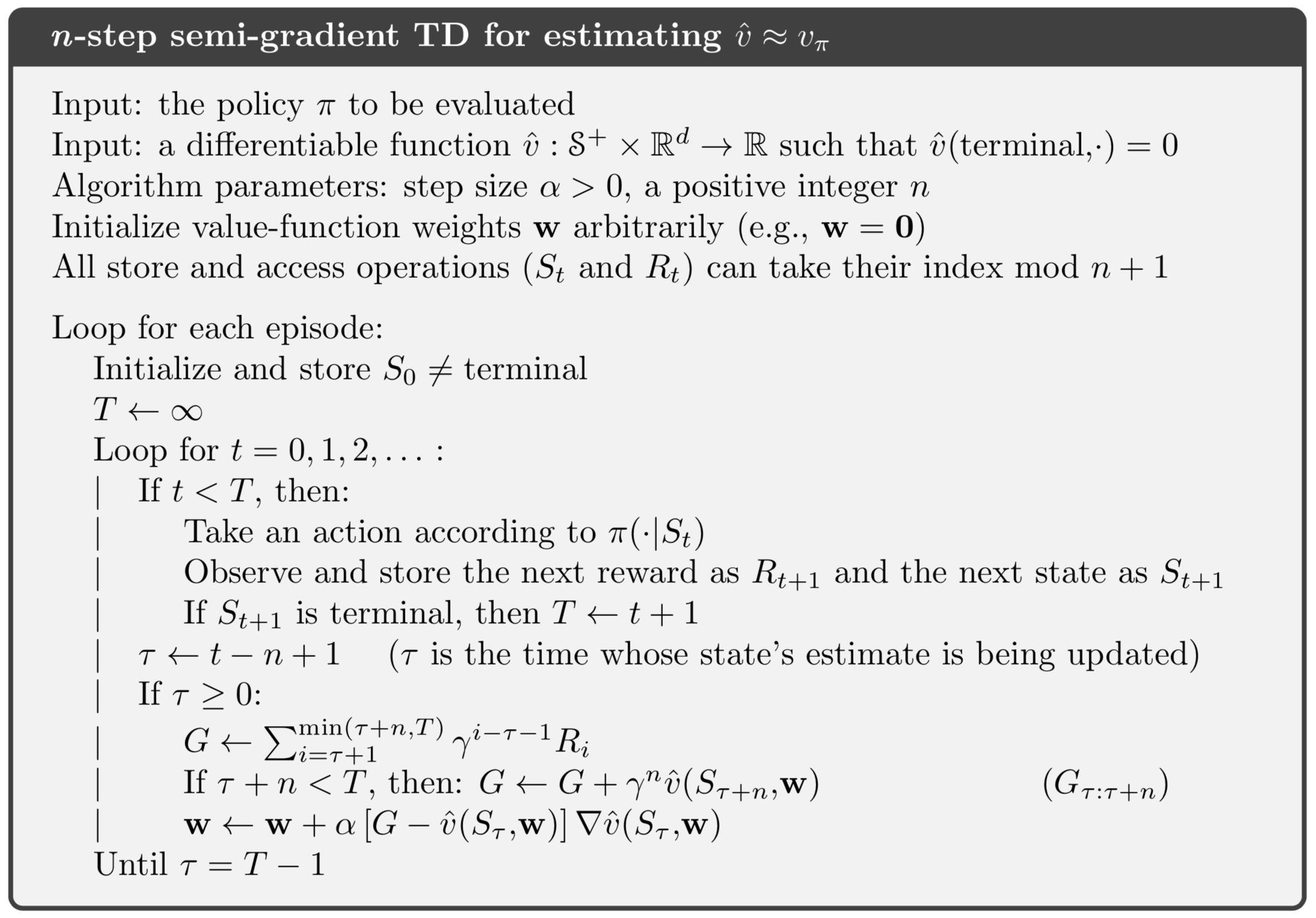
• TD(\(n\)): \(S_t \mapsto G_{t:t+n}\)
• DP: \(S_t \mapsto E_\pi[ R_{t+1} + \gamma v_\pi(S_{t+1}) | S_t = s]\)
• Estimated value shifted toward target
• These relations express input-output relationship for function approximation
• \(s \mapsto u\) means make \(v(s) = u\)
• This is supervised learning!
• Neural networks, regression/decision trees, Gaussian process regression, multivariate regression

Supervised Learning

• Assume: static data

• Perform: multiple passes over data

• Need: online, incremental methods

• Assume: stationary function

• Need: adaptation to time-varying functions

Prediction Objective

• Tabluar case
  • No measure of prediction quality needed
  • Estimated \(v\) able to approch \(v_\ast\) exactly
  • One \(v\) value (in the table) for each state \(s\)
  • \(v(s)\) independent of \(v(s')\)

Prediction Objective

• Approximation
  • \(\hat{v}(s,\mathbf{w})\) not independent of \(\hat{v}(s',\mathbf{w})\)
  • Values linked through \(\mathbf{w}\)
  • Need objective because \(\hat{v}(s,\mathbf{w}) \neq v_\ast(s)\) for all \(s\)
  • Limited parameter set: \(\uparrow \hat{v}(s_0,\mathbf{w})\) leads to \(\downarrow \hat{v}(s_1,\mathbf{w})\)
  • State distribution \(\mu\) expresses how much we care about different states

Prediction Objective

• State distribution \(\mu\): \(\mu(s) \geq 0\) and \(\sum_s \mu(s) = 1\)
• Mean squared error objective: \[ \bar{\text{VE}}(\mathbf{w}) = \sum_s \mu(s) \left[ v_\pi(s) - \hat{v}(s,\mathbf{w}) \right]^2 \]
• On-policy distribution: \(\mu(s)=\) fraction of time spent in \(s\)
• Note: Best MMSE value function not guaranteed to produce best policy, but it gives a useful one

Learning Goal

• Find \(\mathbf{w}^\ast\) for which \(\bar{\text{VE}}(\mathbf{w}^\ast) \leq \bar{\text{VE}}(\mathbf{w})\) for all \(\mathbf{w}\)
• Possible with simple approximators
• Rarely possible with complex approximators
• Settle for local optimality: \[ \bar{\text{VE}}(\mathbf{w}^\ast) \leq \bar{\text{VE}}(\mathbf{w}) \quad \|\mathbf{w} - \mathbf{w}^\ast\| \leq \delta \]

Stochast Gradient Descent

• Assume states appear in examples with distribution \(\mu\). Then minimize error on obsered samples
• SGD adjust \(\mathbf{w}\) by small amount after each observation \[ \begin{align} \mathbf{w}_{t+1} &= \mathbf{w}_t - \alpha \frac{1}{2} \nabla \left[ v_\pi(S_t) - \hat{v}(S_t,\mathbf{w}_t)\right]^2 \\ &= \mathbf{w}_t + \alpha\left[ v_\pi(S_t) - \hat{v}(S_t,\mathbf{w}_t)\right] \nabla \hat{v}(S_t,\mathbf{w}_t) \end{align} \]

Available Information

\[ \mathbf{w}_{t+1} = \mathbf{w}_t + \alpha\left[ U_t - \hat{v}(S_t,\mathbf{w}_t)\right] \nabla \hat{v}(S_t,\mathbf{w}_t) \]

• If \(E[U_t|S_t] = v_\pi(S_t)\) (unbiased), then \(\mathbf{w}\)_t guaranted to converge to local optimimum
• We have followed this pattern many times
• Replace something that we don’t know by something we do know such as an estimate (bootstrap which is biased, DP) or something we can compute from observations (average which is unbiased, MC)

Gradient MC Alg

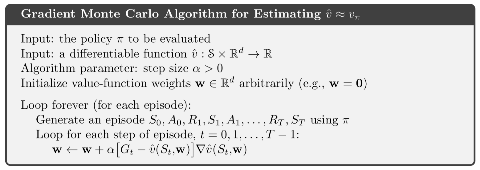
Convergence to local opt is guaranteed.

Semigradient for Bootstrapping

• Bootstrap methods: DP, TD(0), TD(\(n\)) are biased
• Target \(U_t\) depends indirectly on \(\mathbf{w}_t\) but this is not accounted for in the gradient (call them semigradient methods)
• Semigradient offer advantages:
  • Faster learning
  • Continual online learning
  • Don’t have to wait till episode end

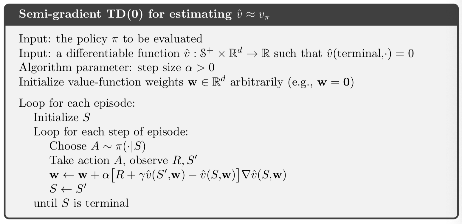
Semigrad TD(0)

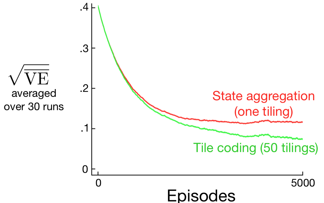
State Agregation

• Lies between tabular methods and full function approximation
• States are grouped together (TBD) with one value for each state in the group
• This is like a piece-wise constant value function
• \(\nabla \hat{v}(S_t,\mathbf{w}_t)=1\) for \(S_t\)’s group and is zero otherwise

Linear Methods

• Feature vector: \(\mathbf{x}(s) = (x_1(s), x_2(s), \cdots, x_d(s))^T\)
• Linear in the weights: \[ \begin{align} \hat{v}(s,\mathbf{w}) &= \mathbf{w}^T \mathbf{x}(s) = \sum_{i=1}^d w_i x_i(s) \\ \nabla \hat{v}(s,\mathbf{w}) &= \mathbf{x}(s) \\ \mathbf{w}_{t+1} &= \mathbf{w}_t + \alpha \left[ U_t - \hat{v}(S_t,\mathbf{w}_t) \right] \mathbf{x}(S_t) \end{align} \]

Convergence Results: Linear Approx.

• Single global optimum of MSE
• SGD-MC guaranteed to converge provided \(\alpha\) decreases over time

Convergence Results: Semi-Gradient TD(0)

• Converges close to local optimum
• Update: \[ \begin{align} \mathbf{w}_{t+1} &= \mathbf{w}_t + \alpha\left[ R_{t+1} + \gamma \mathbf{w}_t^T \mathbf{x}_{t+1} - \mathbf{w}_t^T \mathbf{x}_t\right] \mathbf{x}_t \\ &= \mathbf{w}_t + \alpha\left[ R_{t+1}\mathbf{x}_t - \mathbf{x}_t(\mathbf{x}_t - \gamma \mathbf{x}_{t+1})^T \mathbf{w}_t \right] \end{align} \]

• Steady state: \(E[\mathbf{w}_{t+1} | \mathbf{w}_t] = \mathbf{w}_t+ \alpha(\mathbf{b} - \mathbf{A} \mathbf{w}_t)\) \[ \mathbf{b} = E[R_{t+1}\mathbf{x}_t] \quad \text{and} \quad \mathbf{A} = E[ \mathbf{x}_t(\mathbf{x}_t - \gamma \mathbf{x}_{t+1})^T] \]
• At convergence: \(E[\mathbf{w}_{t+1} | \mathbf{w}_t] = \mathbf{w}_t\) \[ \mathbf{b} - \mathbf{A} \mathbf{w}_\text{TD} = \mathbf{0} \quad \Rightarrow \quad \mathbf{w}_\text{TD} = \mathbf{A}^{-1} \mathbf{b} \]

• Analysis in textbook shows: \[ \bar{\text{VE}}(\mathbf{w}_\text{TD}) \leq \frac{1}{1-\gamma} \min_\mathbf{w} \bar{\text{VE}}(\mathbf{w}) \]
• Can be substantial loss in performance with TD(0)
• But TD(0) has much less variance and faster convergence than MC
• Semigradient-DP also converges to TD fixed point

Exercise 9.1 page 209. How are the tabular methods special cases of linear function approximation. What is \(\mathbf{x}(s)\)?

Concepts

• Add prior domain knowledge into RL
• Features should “correspond to the aspetcs of the state space along which generalization may be appropriate”
• Limitation: Cannot account for interactions between features (feature \(i\) being good only in absence of feature \(j\))

Examples

• Polynomials
• Fourier basis
• Coarse coding
• Radial basis functions

Polynomials

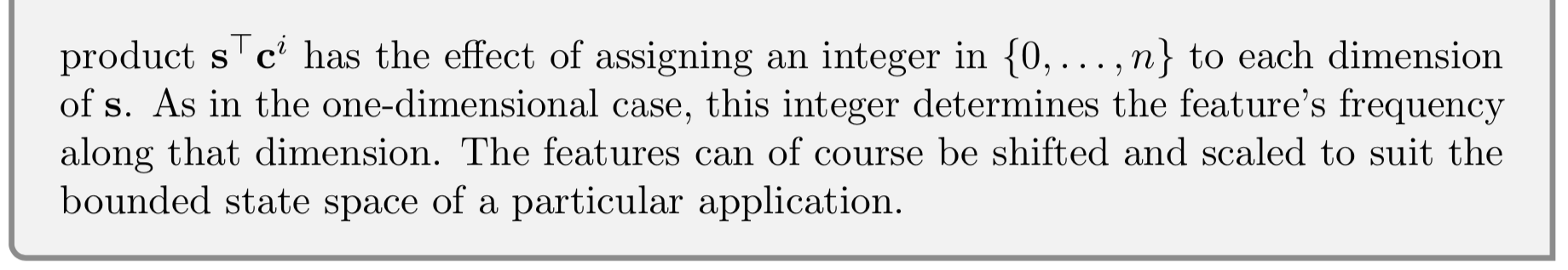
In many problems, states naturally expressed as numbers:

• Positions in 1D, 2D, etc.
• Velocities
• Number of cars in a lot (rental car problem)
• Dollars to invest

Polynomials

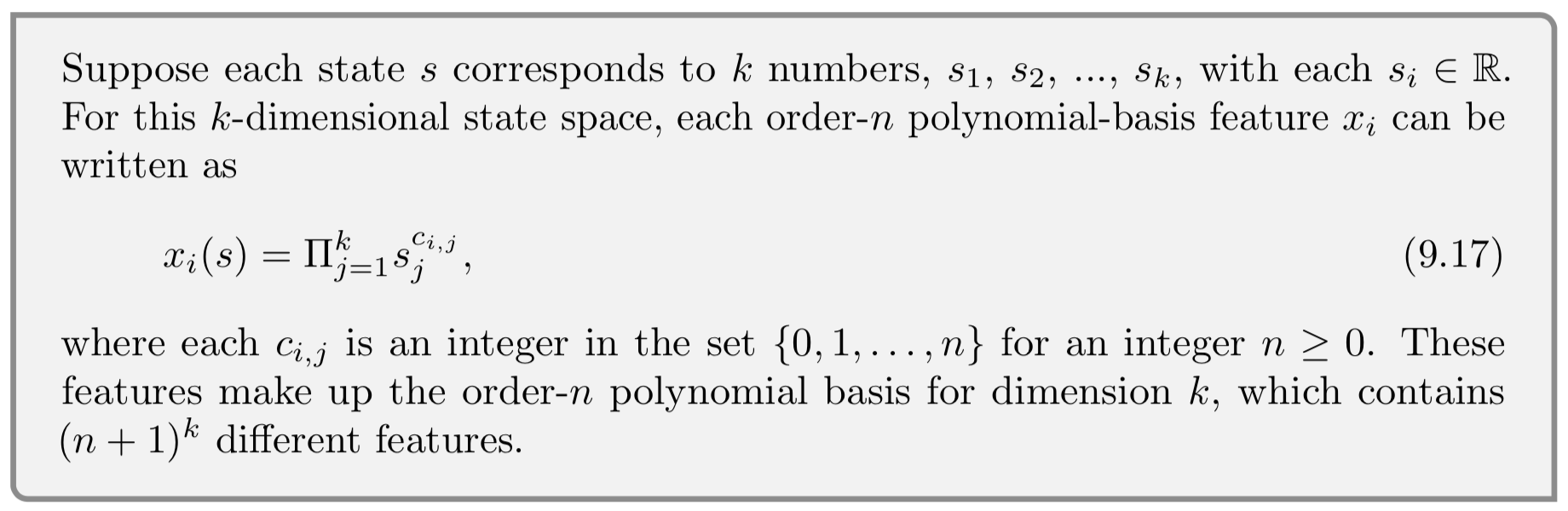
Simple but don’t work as well as other bases.

Fourier Basis

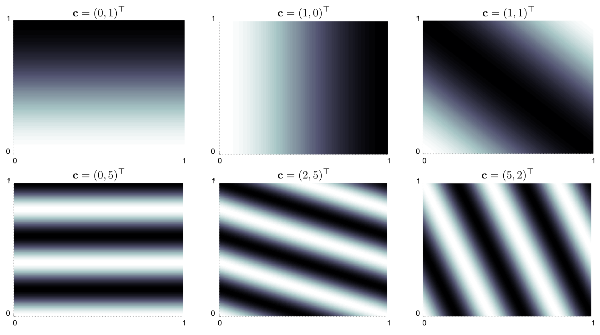
Easy to use and perform well in many RL tasks.

Fourier Basis

Fourier Basis

• Work well for smooth functions
• Can work better than polynomials and RBF
• Gibbs effect at discontinuities

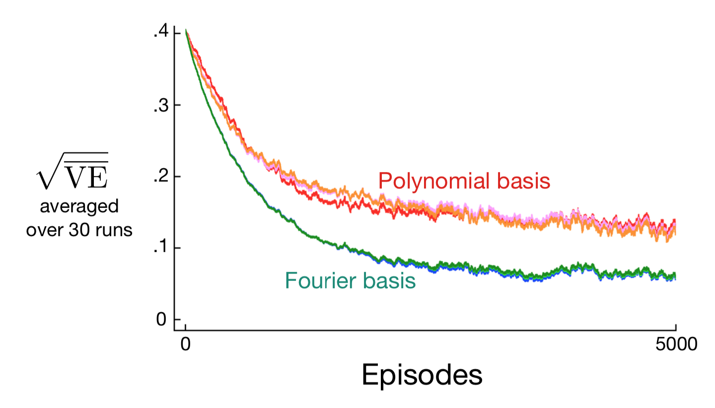
Comparison

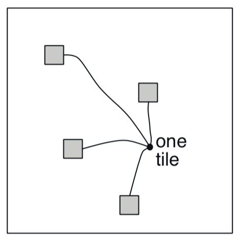
Coarse Coding

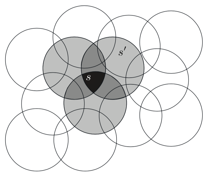
• State space is 2D
• Binary feature: \(x_i(s) = 1\) if \(s\in \mathcal{N_i}\) and is \(0\) else
• \(\mathbf{x}(s)\) is a binary vector
• Need not use circles

Coarse Coding

Without overlap, coarse coding is just state aggregation.

Coarse Coding

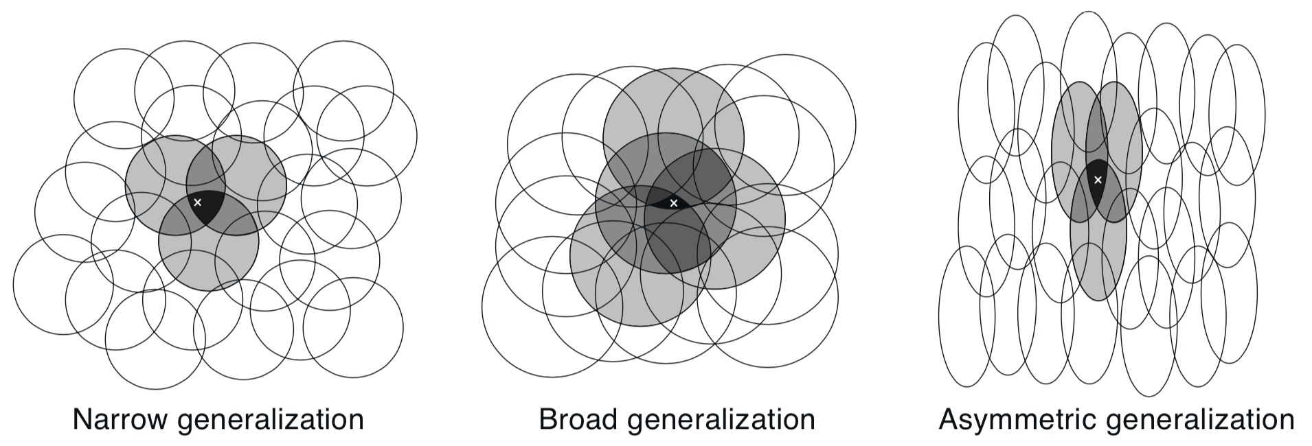
Think about what kind of approximations would arise from linear combinations of binary vectors on these shapes.

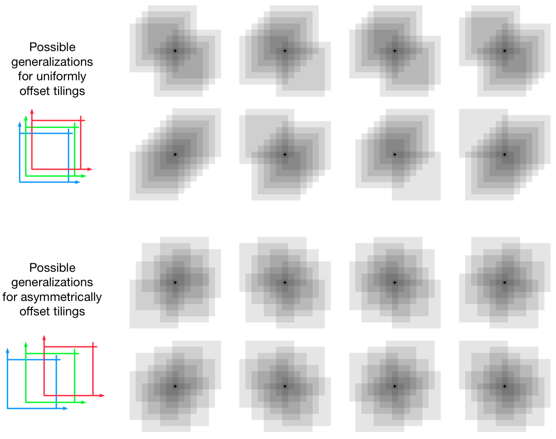
Coarse Coding Example

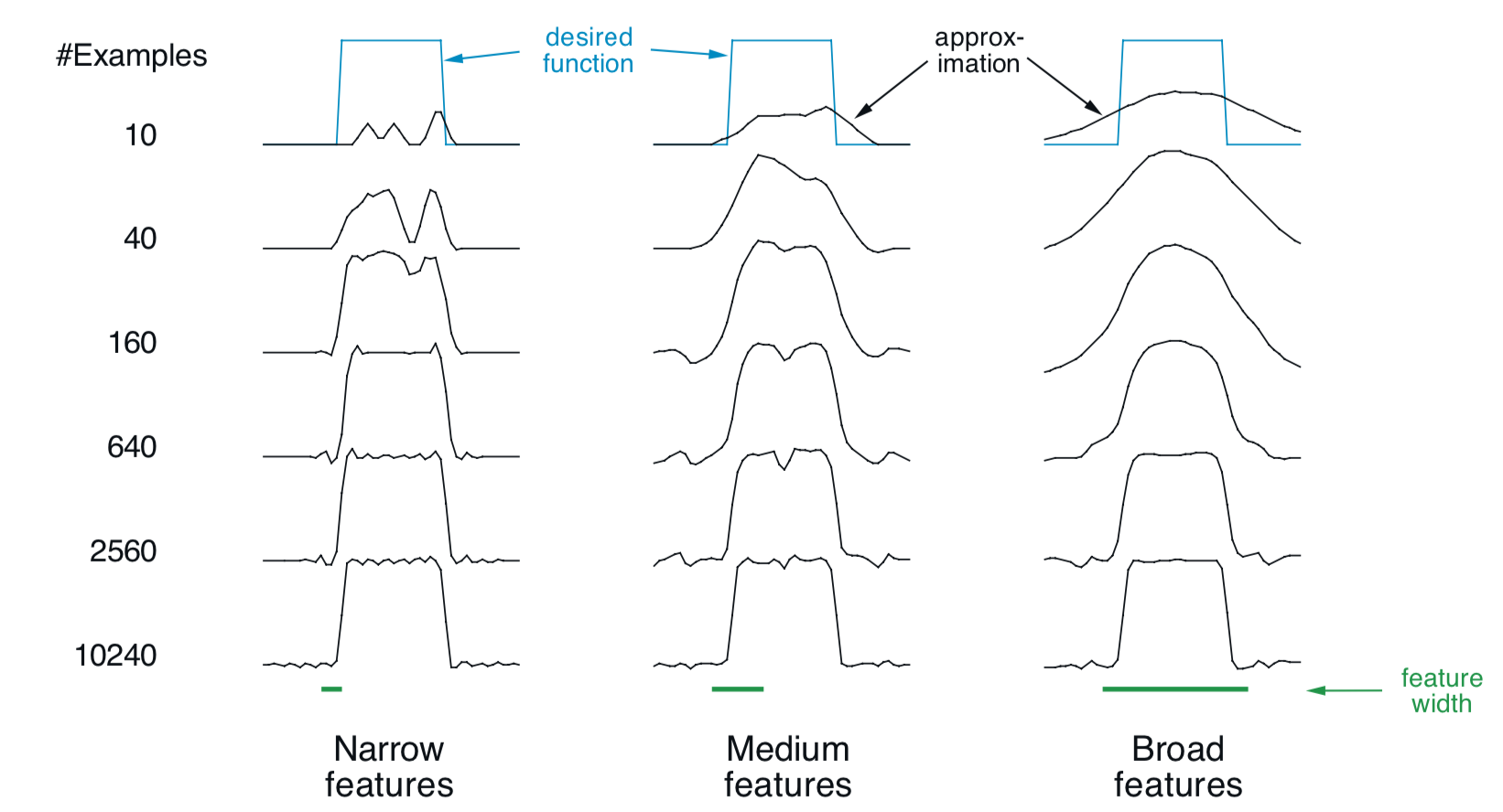
Receptive field shape strong effect on generalization(first row) but little effect on asymptotic approximation quality (last row)

Tile Coding

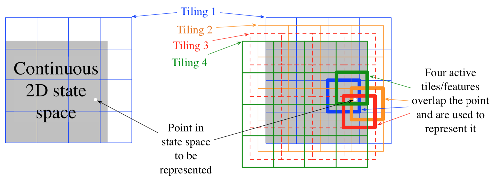
• Tiling = partition
• Multiple \((n)\) offsets
• Each point appears exactly once in each tiling giving gradient updates only \(n \ll d\) weights

Tile Coding

Asymetric offsets

Alternative Partitions

Efficient Hashing

• Hashing = pseudorandom collapsing of large tiling into small set of tiles
• Tiles are noncontiguous, disjoint regions
• Hashing gives a partition
• Memory is reduced
• “Cures” curse of dimensionality

Radial Basis Functions

\[ x_i(s) = \exp\left(-\frac{\|s-c_i\|^2}{2\sigma_i^2}\right) \]

• Softens hard binary 0-1 feature
• Gives smooth and differentiable features

Setting the Step Size

To learn in about \(\tau\) steps, let

\[ \alpha = \frac{1}{\tau E\|\mathbf{x}\|^2} \]

Neural Net Approximators

(You already know about this.)

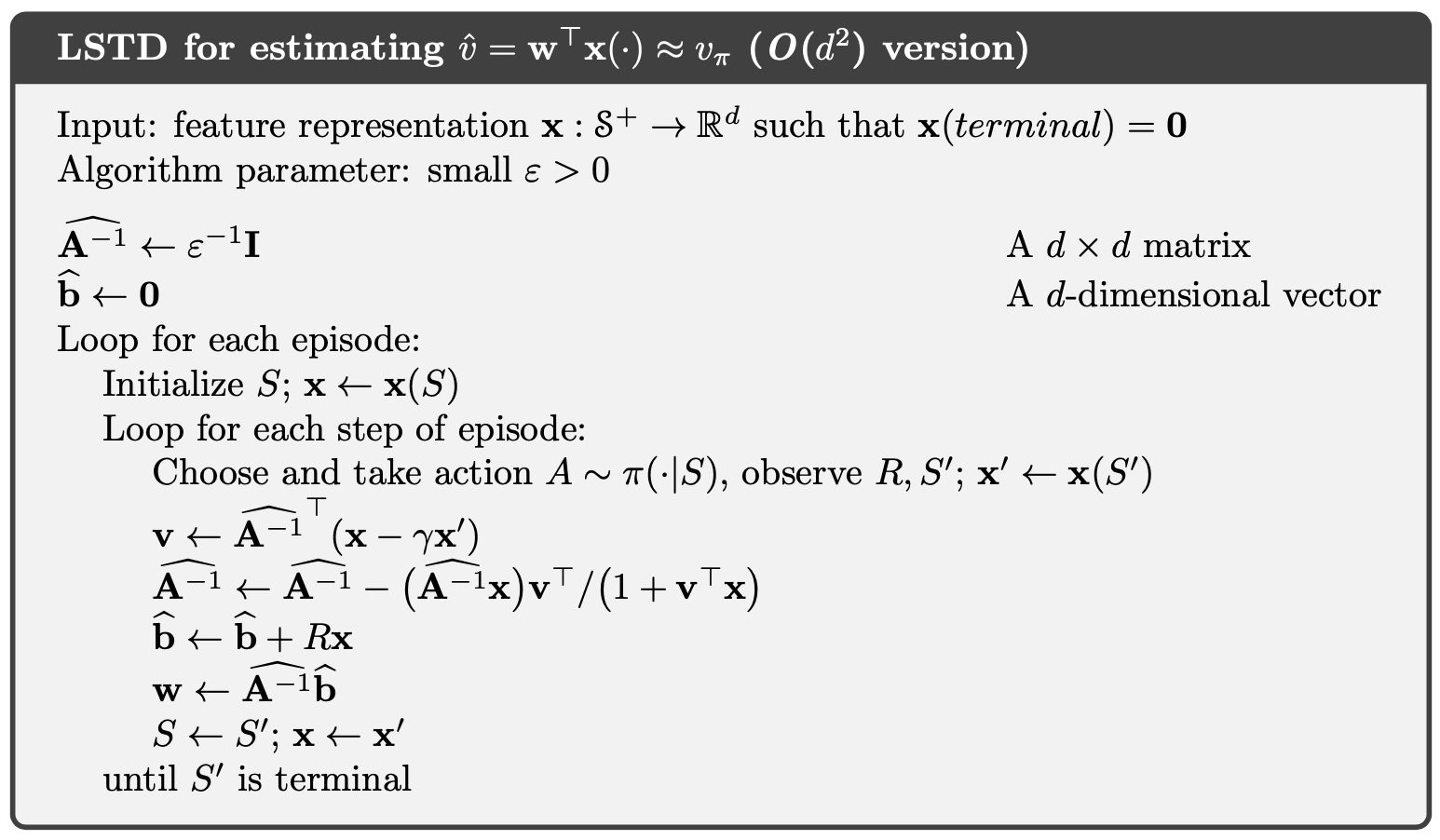
Least-Squares TD (LSTD)

\[ \begin{gather} \mathbf{b} = E[R_{t+1}\mathbf{x}_t] \quad \text{and} \quad \mathbf{A} = E[ \mathbf{x}_t(\mathbf{x}_t - \gamma \mathbf{x}_{t+1})^T] \\ \mathbf{w}_\text{TD} = \mathbf{A}^{-1} \mathbf{b} \end{gather} \]

• TD converges to this solution iteratively
• TD is not data efficient
• LSTD computes this solution directly
• LSTD is data efficient

Sample Averages

\[ \begin{gather} \hat{\mathbf{A}}_t = \sum_{k=0}^{t-1} \mathbf{x}_k (\mathbf{x}_k-\gamma \mathbf{x}_{k+1})^T + \varepsilon \mathbf{I} \qquad \hat{\mathbf{b}}_t = \sum_{k=0}^{t-1} R_{t+1} \mathbf{x}_k \\ \mathbf{w}_t = \hat{\mathbf{A}}_t^{-1} \hat{\mathbf{b}}_t \end{gather} \]

• \(O(d^2)\) memory
• \(O(d^3)\) computation

Matrix Inversion Lemma

\[ \begin{gather} \hat{\mathbf{A}}_{t}^{-1} = \hat{\mathbf{A}}_{t-1}^{-1} - \frac{\hat{\mathbf{A}}_{t-1}^{-1} \mathbf{x}_t (\mathbf{x}_t - \gamma\mathbf{x}_{t+1})^T \hat{\mathbf{A}}_{t-1}^{-1} }{1 + (\mathbf{x}_t - \gamma\mathbf{x}_{t+1})^T \hat{\mathbf{A}}_{t-1}^{-1} \mathbf{x}_t},\;\; \hat{\mathbf{A}}_0 = \varepsilon \mathbf{I} \end{gather} \]

• \(O(d^2)\) memory and computation

LSTD Algorithm

Previous Methods

Previous methods:

• Use single approximating function for \(v_\pi\) over the whole of state space
• Discard data after update to function parameters (parametric)
• Evaluate the approximation function at query states

Memory-Based Approximation

• No parameters, no parameter updates (non-parameteric)
• Save training samples
• Training samples retrieved from memory and used/combined to compute approximated value at query state

Examples

• Nearest neighbor method:
  • \(s' \mapsto g'\) is stored in memory
  • \(s'\) is closest training sample to query state \(s\)
  • target \(g'\) is returned as response to \(s\)
• Extend to weighted average of \(k\) nearest neighbors
• Locally weighted regression
  • Fits surface to targets \(g'\) of training samples \(s'\) closest to query state \(s\)
  • This combines function approximation and memory-based methods
• Gaussian process regression is another example of a memory-based method
  • GPR assumes a joint Gaussian model between training states, training targets, and the query state to estimate the query target

Advantages of Memory-Based Methods

• Not limit approx. to pre-specified functions
• Accuracy improves as data accumulates
• May be no need for global approximation because many areas of state space will never be visited
• Avoiding global approximation addresses curse of dimensionality
• Experience has immediate affect on value estimates in the neighborhood of the current state

Advantages of Memory-Based Methods

• Question: Responding to queries quickly?
• Answer: \(k\)-d tree data structures

Kernel Functions

\[ \hat{v}(s,\mathcal{D}) = \sum_{s' \in \mathcal{D}} k(s,s') g(s') \]

• \(\mathcal{D}\) is the stored training set
• \(g(s')\) is the target at state \(s'\)
• \(k(s,s')\) is the kernel function

Kernel Functions

\[ k(s,s') \]

• Express how relevant knowledge of any state is to any other state
• Weight given to data about \(s'\) in its influence on answering queries about \(s\)
• Measures the strength of generalization from \(s'\) to \(s\)

Kernel Functions

\[ k(s,s') \]

• Gaussian RBF is a popular kernel
• Kernel RBF differs from predetermined set of RBF basis
  • Memory based - RBFs centered on data
  • Non-parametric - No parameters to estimate
• Just calculate \(\hat{v}(s,\mathcal{D}) = \sum_{s' \in \mathcal{D}} k(s,s') g(s')\)