Background

• Combines MC and DP ideas
• Learns from experience like MC
• Bootstraps like DP

MC Prediction

\[ V(S_t) \leftarrow V(S_t) + \alpha[G_t-V(S_t)] \]

• Constant \(\alpha\) suitable for nonstationary env.
• MC updates at end of episode when \(G_t\) known

TD Prediction

\[ V(S_t) \leftarrow V(S_t) + \alpha[R_{t+1} + \gamma V(S_{t+1}) -V(S_t)] \]

• Uses idea that \(V(S_t) = E[G_t|S_t]\) and \(G_t = R_{t+1} + \gamma G_{t+1}\)
• Updates immediately on transition to \(S_{t+1}\) when \(R_{t+1}\) is received
• Does not wait till end of episode
• Called one-step TD or \(TD(0)\)

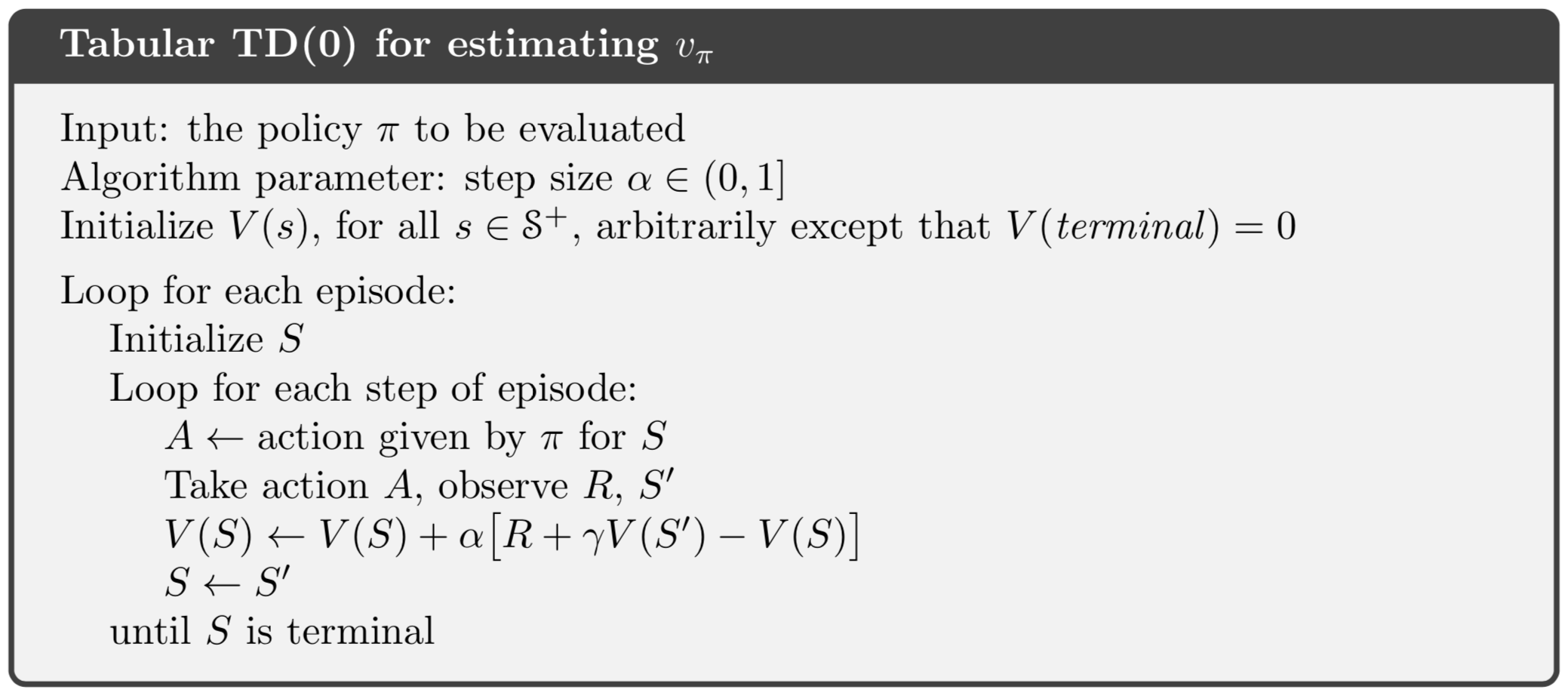
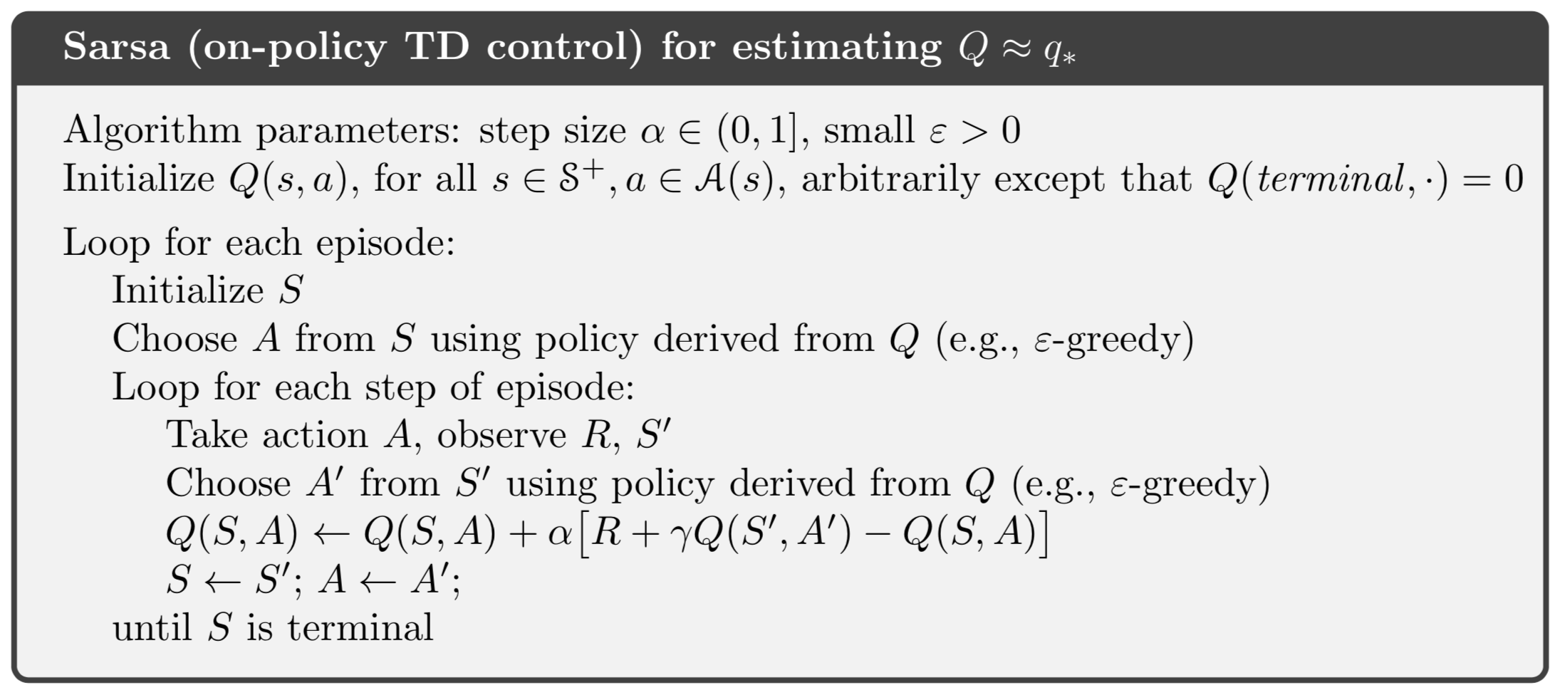
TD Prediction Algorithm

TD(0) Bootstraps

• TD estimate depends on previously estimated value
• Also note relation between MC and TD targets

\[ \begin{alignat}{2} v_\pi(s) &= E_\pi[G_t |S_t=s] \quad & &(\text{MC target}) \\ &= E_\pi[R_{t+1}+ \gamma G_t |S_t=s] \\ &= E_\pi[R_{t+1} + \gamma v_\pi(S_{t+1}) |S_t=s] \quad & &(\text{TD target}) \end{alignat} \]

• TD combines sampling of MC and bootstrap of DP

TD(0) Backup Diagram

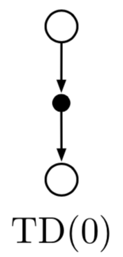
• TD and MC use sample updates
• DP uses expected updates

TD Advantages

• TD bootstraps (like DP, MC doesn’t)
• TD does not requires \(p(s',r|s,a)\) (DP requires it)
• TD is online and incremental (MC updates after episodes)
• TD applies to continuing tasks (MC oriented to episodic tasks)
• TD learns from every transition (MC ignores exploratory episodes)

TD(0) Convergence

For stationary MDP and fixed policy \(\pi\), TD prediction (learning \(v_\pi\))

• Convergence in mean to \(v_\pi\) with \(\alpha\)=constant
• Convergence with prob. 1 with decreasing \(\alpha\)

In practice, TD methods converge faster than constant-\(\alpha\) MC on stochastic tasks

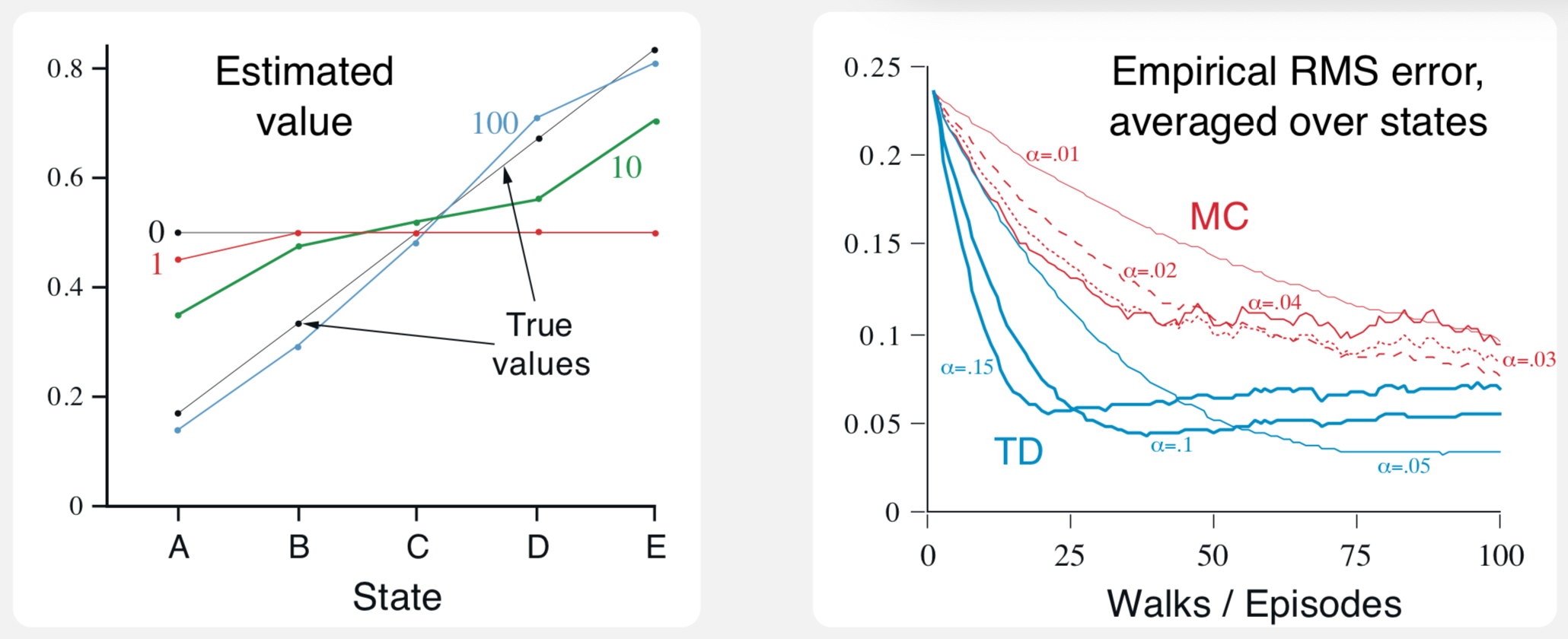
Example 6.2 Random Walk

Homework: Do exercises 6.3 and 6.4 and 6.6.

Batch Update Algorithm

• Finite amount of experience, say, \(N\) episodes
• TD increments computed for every time step
• Value function estimate \(V\) changed only once by sum of increments
• Repeat, process all experience again, etc.
• With small \(\alpha\), TD(0) and MC convergence determinsitically … to different answers!

Example 6.3 Random Walk

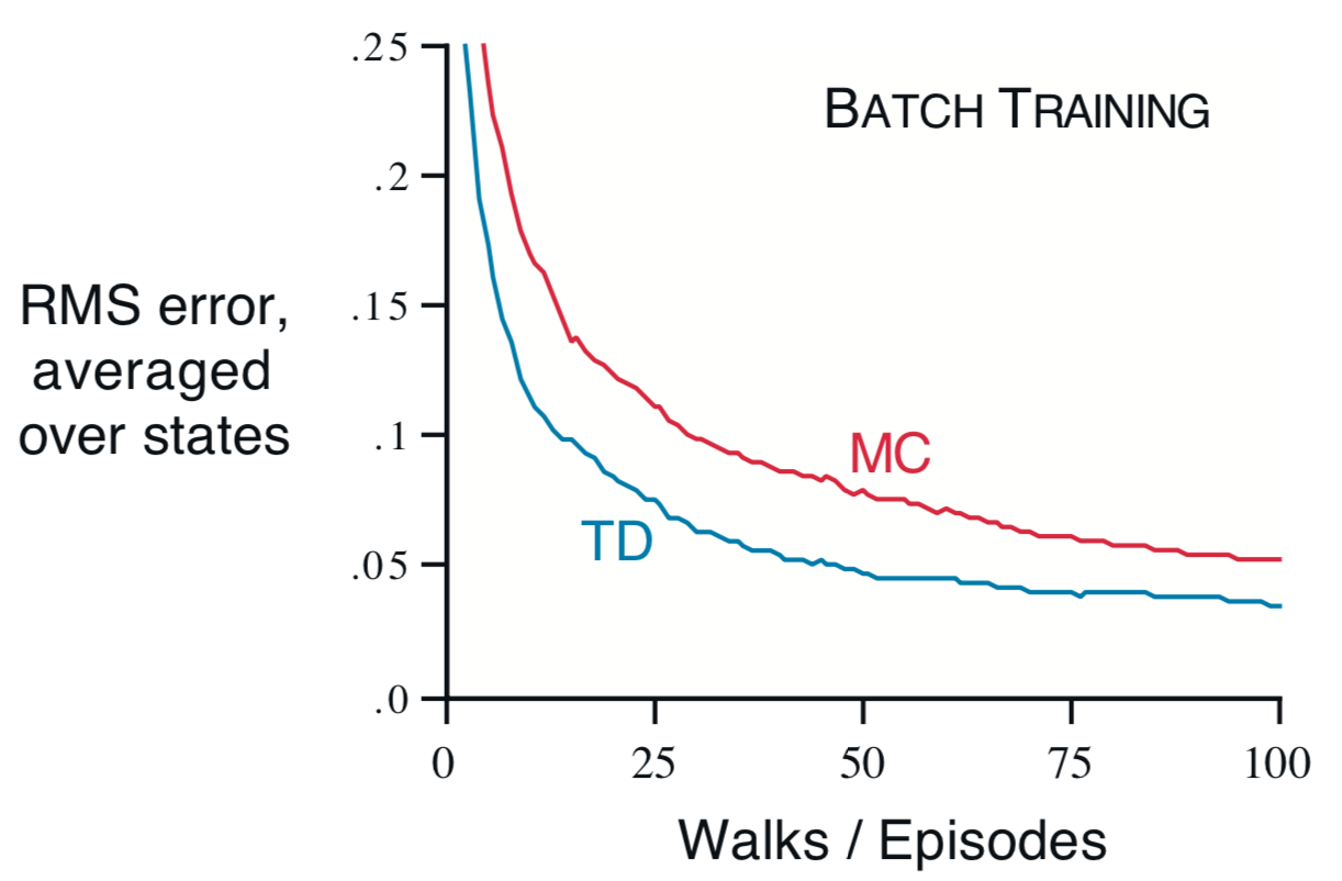
• MC averages actual returns and is optimal (minimizes MSE)
• How does TD perform better?
• TD is optimal in a way that is more relevant to predicting returns

Example 6.4

See example on page 127-128.

What answers do TD and MC give?

Optimality

• Batch MC minimizes MSE on training set
• Batch TD(0) performs ML estimation for Markov model

Certainty-Equivalence Estimate

Given observed episodes:

• \(\hat{p}(s'|s)\)=fraction of observed transitions
• \(\hat{v}_\pi(s)=V(s)\)=average of reward on those transitions

Batch TD(0) converges to the certainty-equivalent estimate (CEE)

Clues to Convergence

• Batch TD(0) faster than MC becuase of CEE
• Non-batch methods do not achieve CEE or MSE, they move in those directions, respectively
• Nonbatch TD(0) faster than constant-\(\alpha\) MC because it is moving toward a better estimate

Exercise & Homework

Start exercise 6.7 (page 128-129) in class and finish as homework.

Background

• Control = Learning optimal policy
• GPI = Prediction (\(\pi_k \rightarrow v_k\)) + Improvement (\(v_k \rightarrow \pi_{k+1}\))
• Use TD methods for prediction
• Trade exploration and exploitation
• On-policy and off-policy
• State value and action value functions

Episode

• Previously considered \(s \rightarrow s'\) transitions and learned value \(v_\pi(s)\) of states
• Now consider \((s,a) \rightarrow (s',a')\) transitions and learn value \(q_\pi(s,a)\) of state-action pairs

SARSA Update

\[ \begin{align} Q(S_t,A_t) \leftarrow& Q(S_t,A_t) \\ &+ \alpha \left[ R_{t+1} + \gamma Q(S_{t+1},A_{t+1}) - Q(S_t,A_t)\right] \end{align} \]

• Update performed immediately after every transition from nonterminal state \(S_t\)
• \(Q(S_{t},A_{t})=0\) if \(S_t\) is terminal
• Uses quintuples \((S_t,A_t,R_{t+1},S_{t+1},A_{t+1})\)

SARSA Backup Diagram

?

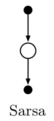
On-Policy SARSA Control

• Estimate \(q_\pi\) (prediction)
• Use \(q_\pi\) as behavior policy
• Change \(\pi\) toward greediness wrt \(q_\pi\) (control)

Convergence of SARSA Control

SARSA converges with prob. 1 to \(\pi_\ast\) provided:

• Policy \(\pi_k\) converges to greedy
• Use \(\varepsilon\)-greedy or \(\varepsilon\)-soft policies with \(\varepsilon = 1/t\)
• Assures all state-action pairs have infinite visits

Exercise 6.8

Do exercise 6.8 (page 129).

Example 6.5 Windy Gridworld

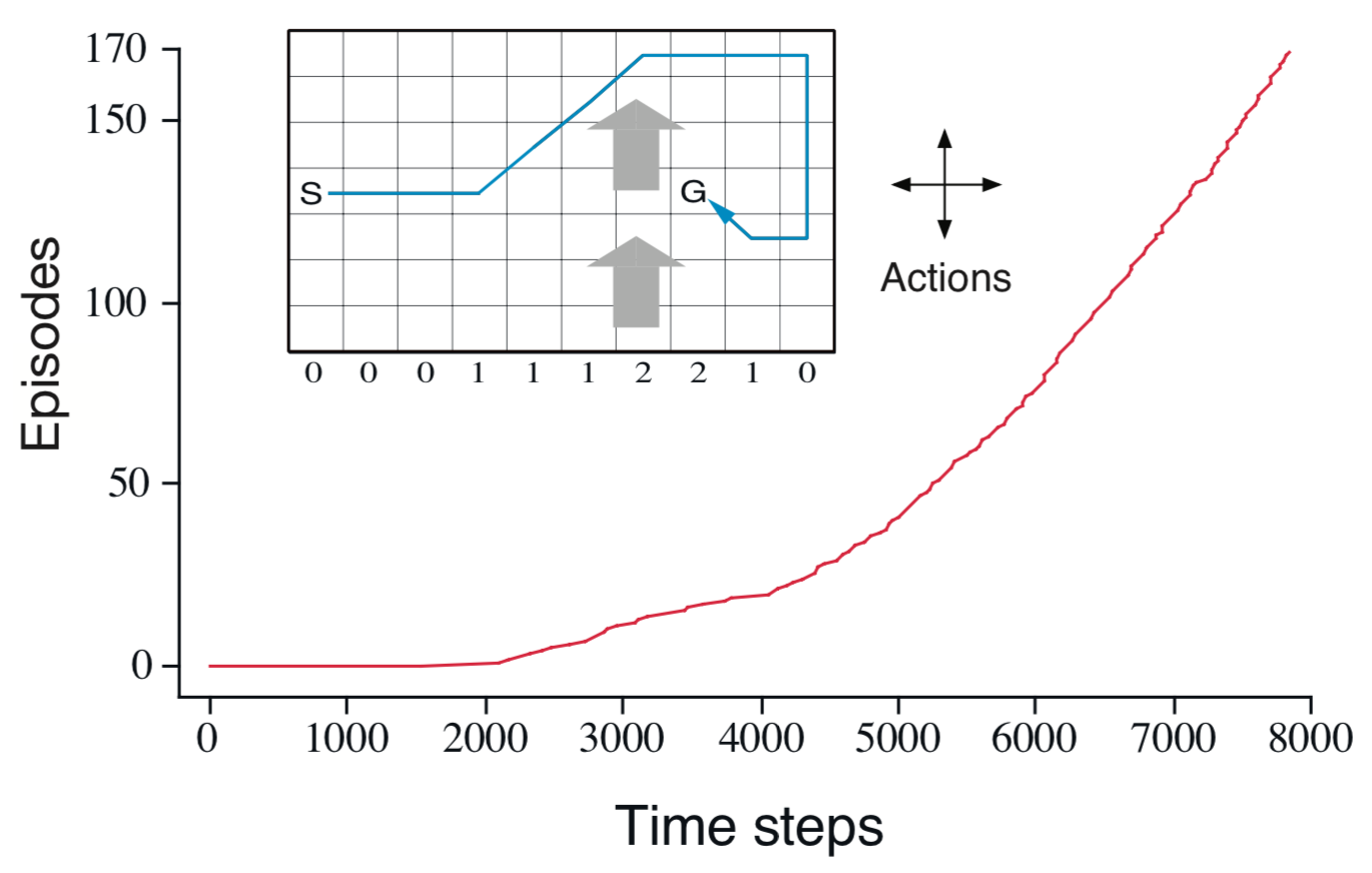
• Discuss example and performance curve
• How can MC fail for this problem?
• See code here

Homework

Do Exercises 6.9 and 6.10 (page 130-131).

Q-Learning

Q-learning = Off-policy TD control

\[ \begin{align} Q(S_t,A_t) \leftarrow& Q(S_t,A_t) \\ &+ \alpha \left[ R_{t+1} + \gamma \max_{a'} Q(S_{t+1},a') - Q(S_t,A_t)\right] \end{align} \]

• Learned \(Q\) approximates \(q_\ast\) independent of behavior policy
• Behavior policy is \(\varepsilon\)-greedy

Convergence

Guaranteed with prob. 1 provide all state-action pairs are visited

Q-Learning Algorithm

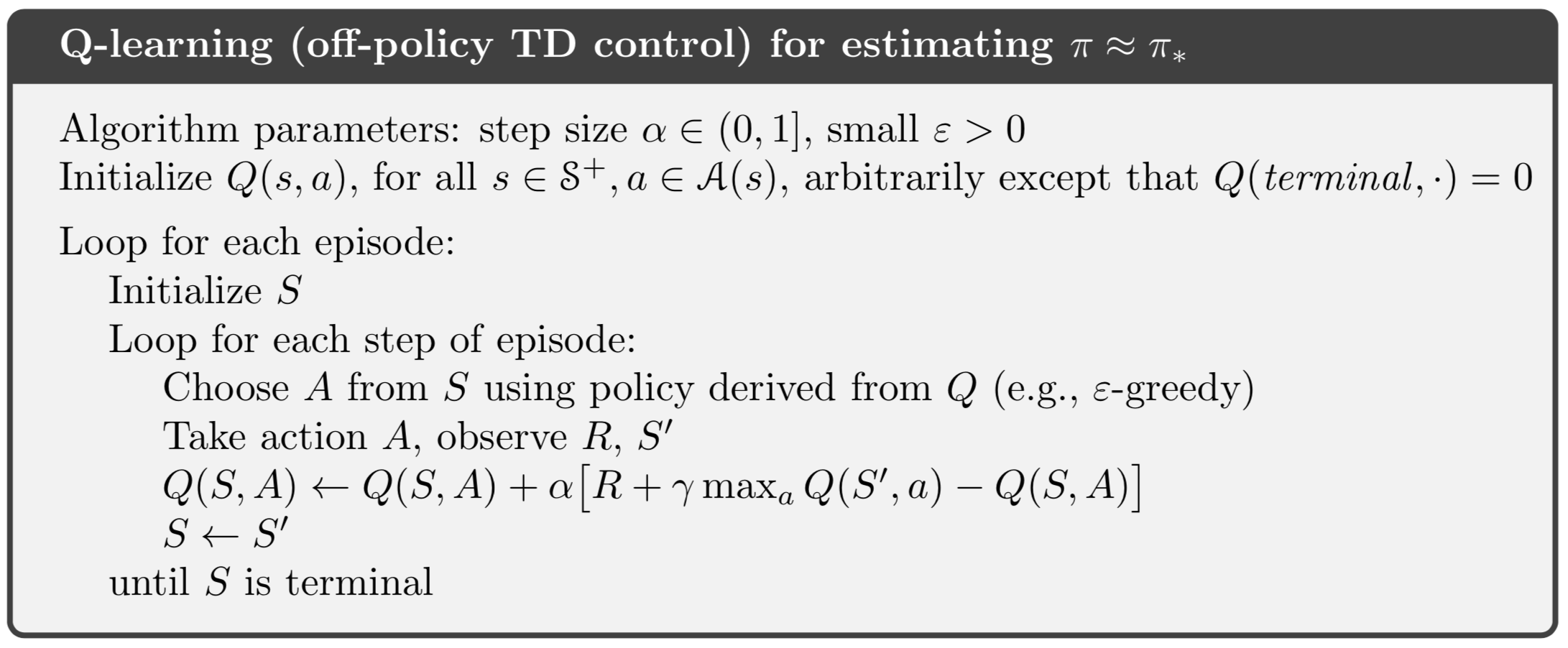
Why is this considered off-policy?

Backup Diagrams

Comparison

• Compare the performance of SARSA and Q-learning in examples 6.6 (page 132).

• Why does SARSA have better rewards?

• Why does SARSA choose the safer path?

SARSA Control Algorithms

\[ \begin{alignat}{2} Q&(S_t,A_t) \leftarrow Q(S_t,A_t) + \alpha [R_{t+1} +& & \gamma \Phi - Q(S_t, A_t)] \\[1em] \Phi &= Q(S_{t+1},A_{t+1}) & & \text{SARSA}\\[1em] \Phi &= \max_{a'}Q(S_{t+1},a') & & \text{Q-learning}\\[1em] \Phi &= \sum_{a'} \pi(a'|S_{t+1})Q(S_{t+1},a') \;\;& & \text{Expected SARSA} \end{alignat} \]

Expected SARSA

\[ \begin{alignat}{2} \Phi &= Q(S_{t+1},A_{t+1}) & & \text{SARSA}\\[1em] \Phi &= \sum_{a'} \pi(a'|S_{t+1})Q(S_{t+1},a') \;\;& & \text{Expected SARSA} \end{alignat} \]

• E-SARSA moves deterministically in the same direction that SARSA moves in expectation
• E-SARSA has lower variance
• Given same amount of experience, E-SARSA should perform better

Comparison

Discussion

• Can do off-policy E-SARSA
• E-SARSA = Q-learning when target policy is greedy
• E-SARSA generalizes Q-learning

Q-Learning is Max. Biased

Why does Q-learning choose left (wrong choice)?

Maximization Bias

• Max of estimated value used as estimate of max of true value
• Max of estiamted value \(>\) max of true value (bias)
• Problem: same data used to determine max action and estimated value
• Solution: Split the data and have two value functions

Double Learning

\[ \begin{align} Q_1(S_t,A_t)&\leftarrow Q_1(S_t,A_t) + \alpha [ R_{t+1} \\ &+\gamma Q_2(S_{t+1},\arg \max_{a'} Q_1(S_{t+1},a')) \\ &- Q_1(S_t,A_t) ] \end{align} \]

Getting the value from \(Q_2\) of the greedy decision from \(Q_1\) to update \(Q_1\) eliminates maximization bias.

Double Learning Algorithm

Homework

• Add a learning curve for E-SARSA to Fig. 6.5 in example 6.7 (page 134-135)
• Do exercise 6.13 on page 136

Tic-Tac-Toe

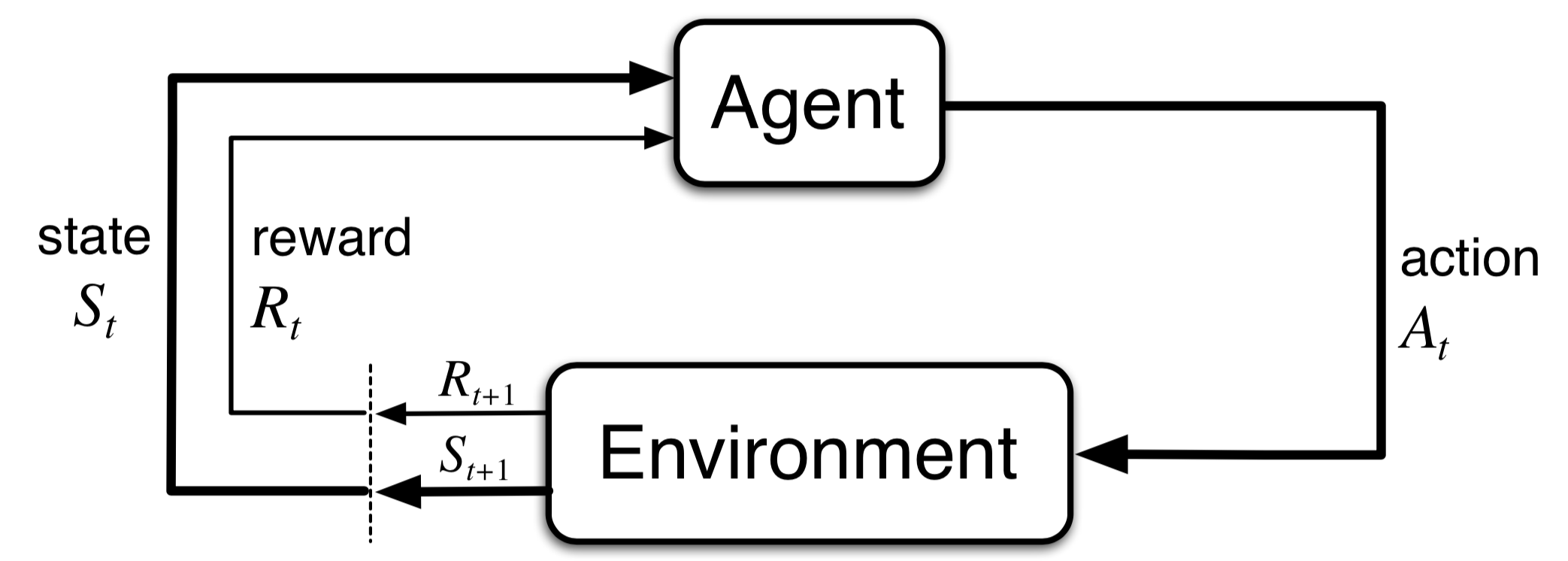
• Discuss tic-tac-toe in the agent-environment setting
• Discuss state vs. “afterstate”
• Discuss state-action vs. position-move
• Why is afterstate-value more efficient than action-value?