Chapter 5: Monte Carlo Methods
Jake Gunther
2019/13/12
Background
Background (1)
- Monte Carlo methods do not use MDP dynamics \(p(s',r|s,a)\)
- Monte Carlo methods learn from experience (state, action, reward) from real or simulated environment
- Can simulate without full knowledge of \(p(s',r|s,a)\)
- Average sample returns
- Chapter 4: Compute \(v_\pi\) from \(\pi\) and \(p\)
- Chapter 5: Learn \(v_\pi\) from \(\pi\) and sample returns
Background (2)
- Episodic tasks (so that we can have many sample trajectories)
- Values and policies changed at end of episodes
Monte Carlo Prediction
Definitions
- Episode under policy \(\pi\): \(S_0, A_0, R_1, S_1, A_1, R_2, \cdots, S_{T-1}, A_{T-1}, R_{T}\)
- Visit to state \(s\): Each occurrence of state \(s\) in episode
- Q: What if \(s\) visited more than once in episode?
- First-visit MC method: \(v_\pi(s)\) = average return following first visit to state \(s\)
- Every-visit MC method: \(v_\pi(s)\) = average returns following all visits to state \(s\)
MC Prediction for \(v_\pi\)
Estimate \(v_\pi(s)\) as the average cumulative future discounted reward starting from state \(s\)
- Prediction
- Policy evaluation: computing/learning \(v_\pi\) consistent with the policy \(\pi\)
- Expected update
MC Prediction Algorithm for \(v_\pi\)
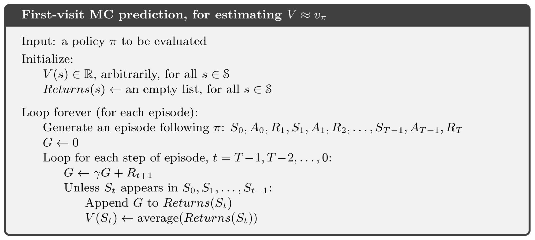
Q: How modify for every-visit MC method?
MC Prediction Algorithm for \(v_\pi\)
- Loop over episodes
- Each visit to state \(s\) yields an iid estimate for \(v_\pi(s)\)
- Law of large numbers predicts convergence to their expected value which is \(v_\pi(s)\)
Example 5.1 Blackjack
- Could not figure out the problem description.
- Q: Why is players sum only 12-21?
- Q: What if player was delat a pair of 2’s?
Advantages/Differences: MC vs. DP
Advantage
- Can have complete knowledge of env. (enough to simulate for MC), but have difficulty formulating \(p(s',r|s,a)\) for DP
- Generating sample episodes is “easy”
- MC can learn from experience (real-world or simulated)
- DP must know full MDP dynamics \(p(s',r|s,a)\)
Backup Diagrams
Dynamic Programming
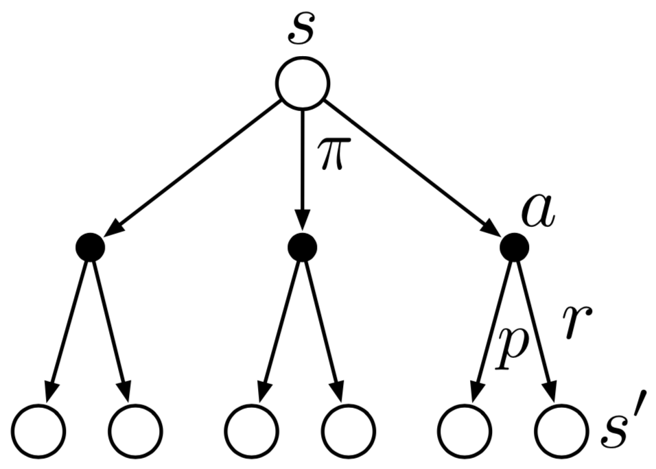
Monte Carlo

Bootstrap
DP: Bellman’s equations update estimates \(v_\pi(s)\) based on other estimates \(v_\pi(s')\)
DP: This is bootstrapping
MC: Estimates \(v_\pi(s)\) are independent for each state
MC: Does not bootstrap. It averages.
Targeted States
- DP: Estimates/updates \(v_\pi(s)\) in all states
- MC: Can estimate \(v_\pi(s)\) in subset of states
MC Estimation of \(q_\pi\)
- Average return afer visit to state-action pair \((s,a)\) in episode
- First vist vs. every visit (quadratic convergence)
- For deterministic \(\pi\) some \((s,a)\)-pairs may never be visited
- Need to maintain exploration
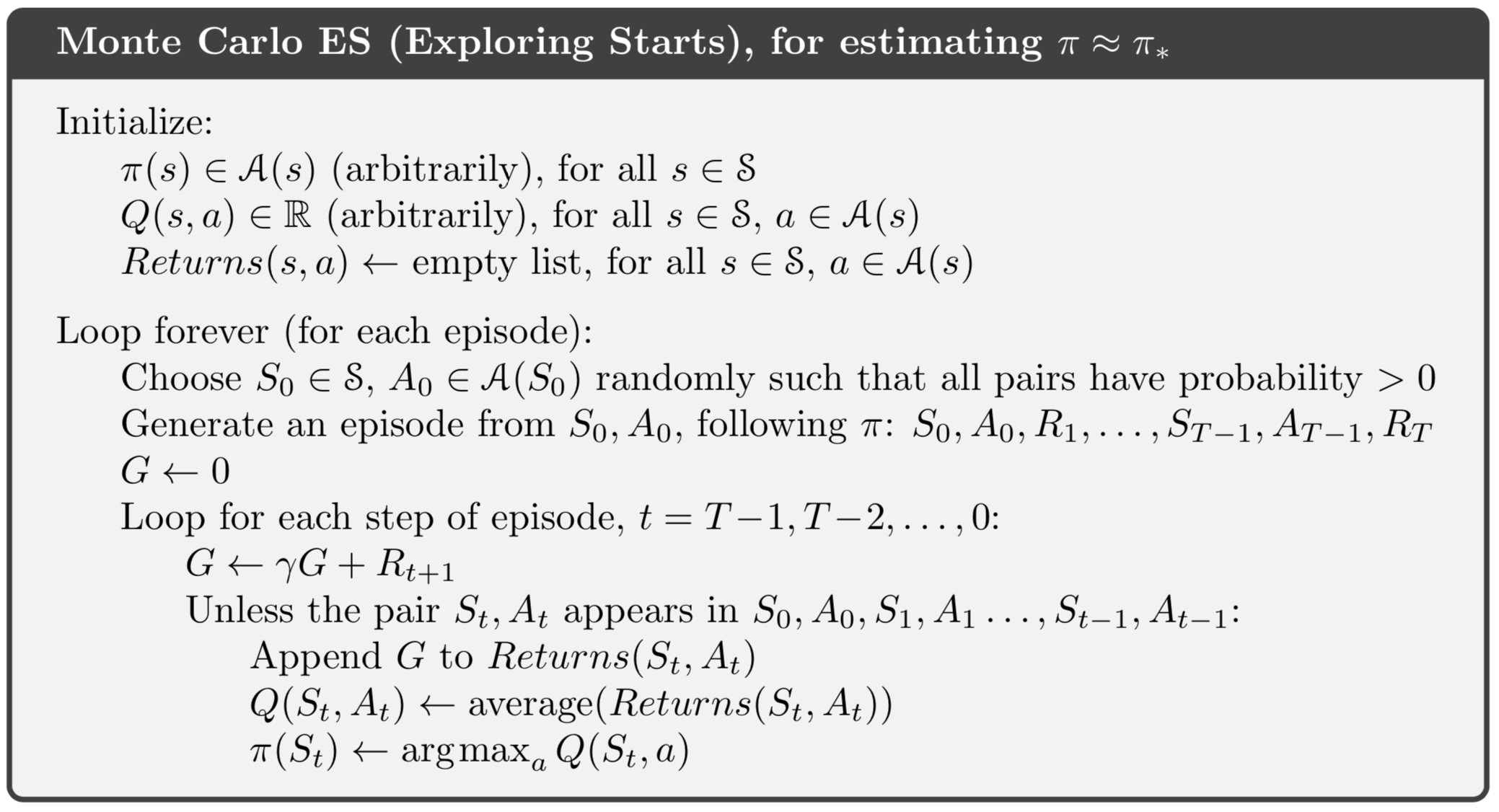
- Exploring starts (ES): Every initial \((s,a)\) has non-zero probability
MC Estimation of \(q_\pi\)
After each episode, alternate between:
- Prediction/estimation: \(\pi_k \rightarrow q_{\pi_k}\)
- Policy evaluation
- Expectation/averaging
- Improvement/control: \(q_{\pi_k} \rightarrow \pi_{k+1}\)
- Can only improve in \((s,a)\) visited during the episode
- ES guarantees that eventually every \((s,a)\) visited
MC Algorithm for \(q_\pi\)
On-Policy vs. Off-Policy
On-Policy vs. Off-Policy
- Want to dispense with exploring starts
- Agent should choose all actions infinitely often in each state
- On-policy: Evaluate and improve the policy used to make decisions
- Off-policy: Evaluate and improve a policy different from the one used to make decisions and generate episodes
- Target policy: policy being learned
- Behavior policy: policy that generates episodes
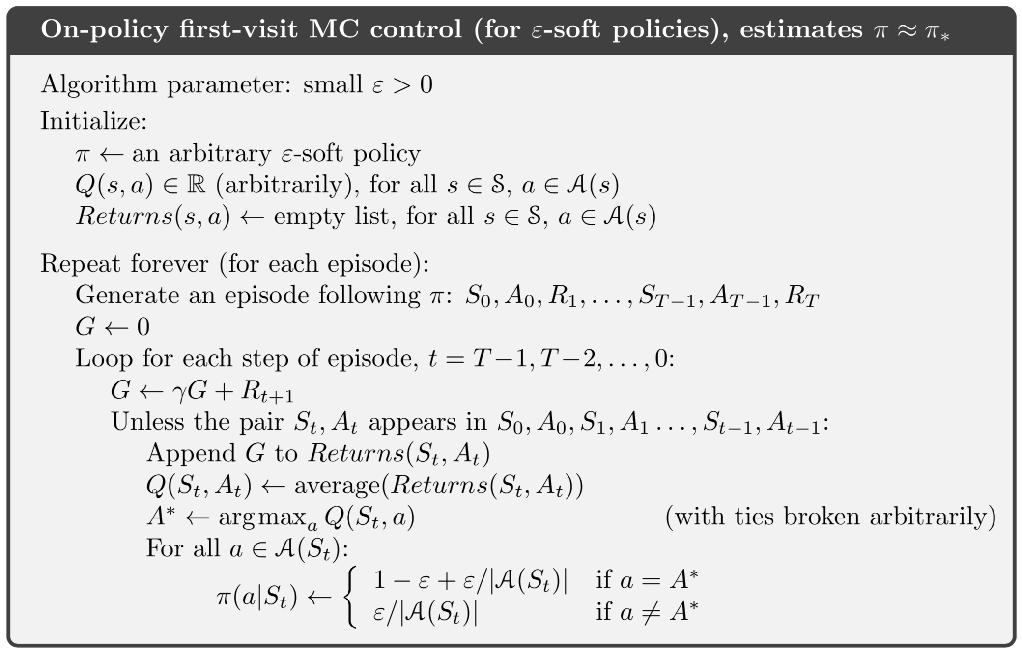
On-Policy Soft Learning
- \(\pi(a|s) >0\) for all \(s\in\mathcal{S}\) and \(a\in\mathcal{A}(s)\)
- \(\varepsilon\)-greedy policy an example of \(\varepsilon\)-soft policy \[ \pi(a|s) = \begin{cases} \frac{\varepsilon}{|\mathcal{A}(s)|}, & \text{non-greedy actions} \\ 1-\varepsilon + \frac{\varepsilon}{|\mathcal{A}(s)|}, &\text{greedy action} \end{cases} \]
Importance Sampling
Background
- Episodes are generated using behavior policy \(b \neq \pi\)
- Suppose all policies are fixed
- Q: How estimate \(v_\pi\) and \(q_\pi\) for target policy \(\pi\)?
- A: Require “coverage”: \[ \pi(a|s) > 0 \quad \Rightarrow\quad b(a|s) > 0 \]
- Target policy can be deterministic/greedy (exploit)
- Behavior policy generally stochastic such as \(\varepsilon\)-greedy (explore)
State-Action Trajectory Prob.
\[ \begin{align} \text{Pr}\{ & A_t, S_{t+1}, \cdots, S_T |S_t,A_{t:T-1} \sim \pi \} \\ &= \prod_{k=t}^{T-1} \pi(A_k|S_k) p(S_{k+1}|S_k,A_k) \end{align} \]
Importance Sampling Ratio
\[ \begin{align} \rho_{t:T-1} &= \frac{\prod_{k=t}^{T-1} \pi(A_k|S_k) p(S_{k+1}|S_k,A_k)}{\prod_{k=t}^{T-1} b(A_k|S_k) p(S_{k+1}|S_k,A_k)} \\ &= \frac{\prod_{k=t}^{T-1} \pi(A_k|S_k)}{\prod_{k=t}^{T-1} b(A_k|S_k)} \end{align} \]
Don’t have to know MDP dynamics \(p(s',r|s,a)\)
Importance Sampling
- Estimate expected values under one distribution given samples from another distribution
- Under behavior policy: \[ E[G_t|S_t=s] = v_b(s) \neq v_\pi(s) \]
- But under behaivor policy: \[ E[\rho_{t:T-1}G_t|S_t=s] = v_\pi(s) \]
Importance Sampling (IS) Conclusion
- Episode state-action trajectories generated by behavior policy \(b\)
- Averages will converge to expectation wrt \(b\) policy
- Averages of importance sampling ratio converge to value of target policy
Implementing IS
- Following S&B notation
- Index time \(t\) across episodes sequentially
- \(T(t)\) = terminiation time following \(t\)
- \(\mathcal{T}(s)\) = set of times when \(s\) is visited
- \(G_t\) = return after \(t\) up to \(T(t)\) (episode end)
- \(\{G_t\}_{t\in\mathcal{T}(s)}\) = returns for state \(s\)
- \(\{\rho_{t:T(t)-1}\}_{t\in\mathcal{T}(s)}\) = IS ratios for state \(s\)
Implementing IS
\[ \begin{align} v_\pi(s) &= E[G_t | S_t=s] \\ V(s) &= \frac{\sum_{t\in\mathcal{T}(s)} \rho_{t:T(t)-1} G_t}{|\mathcal{T}(s)|} \quad (\text{ordinary IS}) \\ &= \frac{\sum_{t\in\mathcal{T}(s)} \rho_{t:T(t)-1} G_t}{\sum_{t\in\mathcal{T}(s)} \rho_{t:T(t)-1}} \quad (\text{weighted IS}) \end{align} \]
First Visit Methods
- Note: \(\rho_{t:T(t)-1}\) can be unbounded
Ordinary IS
- Unbiased
- Variance is unbounded
- Easier to extend to approximate methods
Weighted IS
- Bias \(\rightarrow 0\)
- Variance \(\rightarrow 0\)
- In practice, preferred for lower variance
Every Visit Methods
- Biased for both ordinary and weighted IS
- Bias \(\rightarrow 0\)
- In practice, every-visit method preferred (simpler)
- Every visit easier to extend to approximate methods
Example 5.4
Blackjack: Off policy, single state
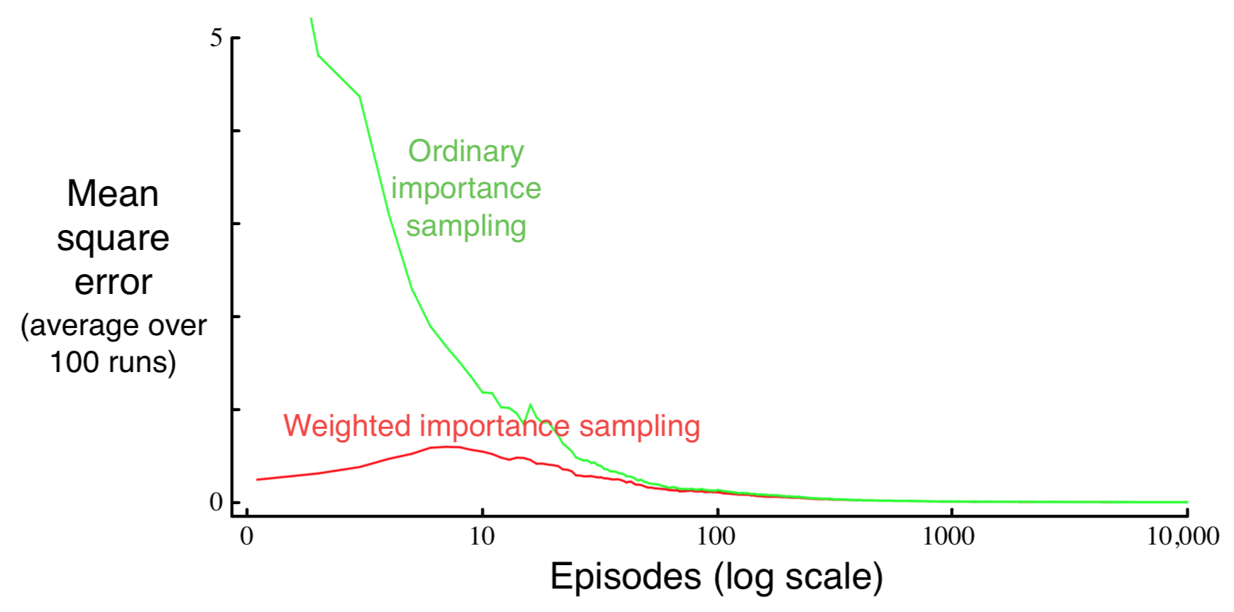
Why the “bump” in the weighted IS curve?
IS for \(q_\pi\)?
\[ \begin{align} q_\pi(s,a) &= E[G_t|S_t=s,A_t=a] \\ Q(s,a) &= ? \end{align} \]
Hints
- Go back to equations for \(V(s)\) and look for \(s\)
- Define \(\mathcal{T}(s) \rightarrow \mathcal{T}(s,a)\)
IS Incremental Implementation
IS Incremental Implementation
\[ \begin{align} V_n = \frac{\sum_{k=1}^{n-1} W_kG_k}{\sum_{k=1}^{n-1} W_k} &= \frac{\sum_{k=1}^{n-1} W_kG_k}{C_{n-1}}, \quad W_i = \rho_{t_i:T(t_i)-1} \\ V_{n+1} C_n &= W_nG_n + V_n C_{n-1} \\ V_{n+1} C_n &= W_nG_n + V_n [C_{n}-W_n] \\ V_{n+1} &= V_n + \frac{W_n}{C_n}[G_n-V_n] \end{align} \]
Off-Policy Prediction

Off-Policy Control
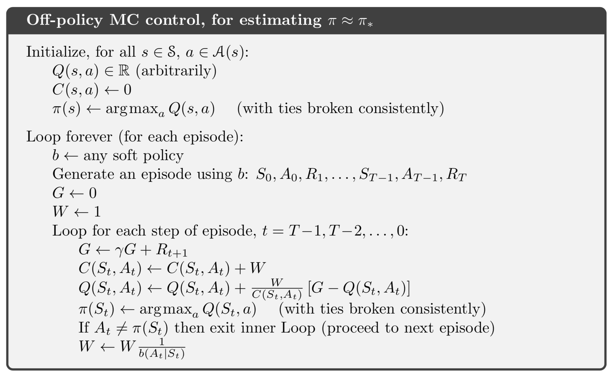
Note Update Structure
\[ Q(S_t,A_t) \leftarrow Q(S_t,A_t) + \alpha [G - Q(S_t,A_t)] \]
- \(G\) is like a target
- \(G-Q(S_t,A_t)\) is the error the points to the target
- \(\alpha\) is a step size
- The overall equation updates to reduce the error, moving \(Q(S_t,A_t)\) closer to the observed target \(G\)
Homework
Do exercise 5.12 on pages 111-112.