Chapter 4 Notes

$v_\pi$

$v_\pi$ instead of solving Bellman's equations as a linear system of equations. (See original code here.)


xxxxxxxxxx
% ... reuse code that sets up p(s',r|s,a) from Chapter 3
% Inplace policy evaluation (prediction) for v_pi
num_iter = 100;  % Maximum number of iterations
v = zeros(25,1); % Initial value function
for iter = 1:num_iter
    vold = v; % Save to test for convergence
    for i=1:5
        for j=1:5
            s = (i-1)*5 + j;
            vs = 0; % Accumulator for inplace computation
            for a=1:4
                for ip=1:5
                    for jp=1:5
                        sp = (ip-1)*5 + jp;
                        for r=1:4
                            % Compute expectation suggested by Bellman's equation
                            vs = vs + 0.25 * p(sp,r,s,a) * (R(r) + gamma*v(sp));
                        end
                    end
                end
            end
            v(s) = vs; % Inplace assignment
        end
    end
    err = norm(v-vold,1); % Compute size of update
    fprintf('iter = %3d, |v-vold| = %10.8f\n',iter,err);
    if(err < 0.01) % Test for termination
        break;
    end
end

Here is the output:


xxxxxxxxxx
iter =   1, |v-vold| = 27.62459555
iter =   2, |v-vold| = 10.16786506
iter =   3, |v-vold| = 5.71330933
iter =   4, |v-vold| = 3.29504090
iter =   5, |v-vold| = 1.96247912
iter =   6, |v-vold| = 1.22910789
iter =   7, |v-vold| = 0.83593787
iter =   8, |v-vold| = 0.65833058
iter =   9, |v-vold| = 0.55351745
iter =  10, |v-vold| = 0.48344337
iter =  11, |v-vold| = 0.43265023
iter =  12, |v-vold| = 0.37922873
iter =  13, |v-vold| = 0.32782581
iter =  14, |v-vold| = 0.28069078
iter =  15, |v-vold| = 0.23871155
iter =  16, |v-vold| = 0.20202362
iter =  17, |v-vold| = 0.17036710
iter =  18, |v-vold| = 0.14329432
iter =  19, |v-vold| = 0.12028819
iter =  20, |v-vold| = 0.10082764
iter =  21, |v-vold| = 0.08442181
iter =  22, |v-vold| = 0.07062582
iter =  23, |v-vold| = 0.05904626
iter =  24, |v-vold| = 0.04934076
iter =  25, |v-vold| = 0.04121476
iter =  26, |v-vold| = 0.03441677
iter =  27, |v-vold| = 0.02873334
iter =  28, |v-vold| = 0.02398405
iter =  29, |v-vold| = 0.02001685
iter =  30, |v-vold| = 0.01670394
iter =  31, |v-vold| = 0.01393805
iter =  32, |v-vold| = 0.01162928
iter =  33, |v-vold| = 0.00970236

$v_\pi$ as solving Bellman's equations as a linaer system.

$q_\pi$

$q_\pi$ .


xxxxxxxxxx
% ... reuse code that sets up p(s',r|s,a) from Chapter 3
% Inplace policy evaluation (prediction) for q_pi
num_iter = 100; % Maximum number of iterations
q = zeros(25,4); % Initial value function
for iter = 1:num_iter
    qold = q; % Save to test for convergence
    for i=1:5
        for j=1:5
            s = (i-1)*5 + j;
            for a=1:4
                qsa = 0; % Accumulator for inplace computation
                for ip=1:5
                    for jp=1:5
                        sp = (ip-1)*5 + jp;
                        for r=1:4
                            % Compute expectation suggested by Bellman's equation
                            qsa = qsa + p(sp,r,s,a)*(R(r) + gamma*0.25*sum(q(sp,:)));
                        end
                    end
                end
                q(s,a) = qsa; % Inplace assignment
            end
        end
    end
    err = sum(sum(abs(q-qold))); % Compute size of update
    fprintf('iter = %3d, |q-qold| = %10.8f\n',iter,err);
    if(err < 0.01) % Test for termination
        break;
    end
end

Here is the output:


xxxxxxxxxx
iter =   1, |q-qold| = 123.36041637
iter =   2, |q-qold| = 53.58055428
iter =   3, |q-qold| = 26.93173329
iter =   4, |q-qold| = 14.48878524
iter =   5, |q-qold| = 7.97903765
iter =   6, |q-qold| = 4.81052880
iter =   7, |q-qold| = 3.27817039
iter =   8, |q-qold| = 2.64359683
iter =   9, |q-qold| = 2.34263687
iter =  10, |q-qold| = 2.05074371
iter =  11, |q-qold| = 1.74947287
iter =  12, |q-qold| = 1.46812616
iter =  13, |q-qold| = 1.21869089
iter =  14, |q-qold| = 1.00418227
iter =  15, |q-qold| = 0.82320700
iter =  16, |q-qold| = 0.67242938
iter =  17, |q-qold| = 0.54787302
iter =  18, |q-qold| = 0.44557900
iter =  19, |q-qold| = 0.36191219
iter =  20, |q-qold| = 0.29367901
iter =  21, |q-qold| = 0.23814762
iter =  22, |q-qold| = 0.19302073
iter =  23, |q-qold| = 0.15638828
iter =  24, |q-qold| = 0.12667448
iter =  25, |q-qold| = 0.10258628
iter =  26, |q-qold| = 0.08306671
iter =  27, |q-qold| = 0.06725406
iter =  28, |q-qold| = 0.05444723
iter =  29, |q-qold| = 0.04407654
iter =  30, |q-qold| = 0.03567962
iter =  31, |q-qold| = 0.02888143
iter =  32, |q-qold| = 0.02337794
iter =  33, |q-qold| = 0.01892282
iter =  34, |q-qold| = 0.01531649
iter =  35, |q-qold| = 0.01239732
iter =  36, |q-qold| = 0.01003444
iter =  37, |q-qold| = 0.00812186

Here is the solution.

s	$q(s,\text{up})$	$q(s,\text{down})$	$q(s,\text{right})$	$q(s,\text{left})$
1	1.9786	1.3699	7.9108	1.9785
2	8.7897	8.7897	8.7897	8.7897
3	2.9853	2.0255	4.7905	7.9107
4	5.3227	5.3227	5.3227	5.3227
5	0.3434	0.4930	0.3433	4.7905
6	2.9785	0.0462	2.6935	0.3698
7	7.9107	0.6648	2.0255	1.3698
8	3.9852	0.6062	1.7172	2.6934
9	4.7905	0.3227	0.4930	2.0255
10	1.3433	-0.3625	-0.5070	1.7171
11	1.3698	-0.8758	0.6648	-0.9539
12	2.6934	-0.3916	0.6062	0.0461
13	2.0255	-0.3190	0.3227	0.6647
14	1.7171	-0.5267	-0.3625	0.6061
15	0.4929	-1.0645	-1.3625	0.3227
16	0.0461	-1.6715	-0.3916	-1.8759
17	0.6647	-1.2103	-0.3190	-0.8759
18	0.6061	-1.1060	-0.5267	-0.3916
19	0.3227	-1.2803	-1.0645	-0.3191
20	-0.3626	-1.7774	-2.0645	-0.5268
21	-0.8759	-2.6716	-1.2103	-2.6716
22	-0.3916	-2.2104	-1.1060	-1.6716
23	-0.3191	-2.1060	-1.2803	-1.2104
24	-0.5268	-2.2803	-1.7774	-1.1061
25	-1.0645	-2.7774	-2.7774	-1.2804

$q_\pi$ $v_\pi$ ?

$v_\pi(s)$ $q_\pi(s,a)$ ?

Do the solutions agree mathematically? Do some spot checking using hand calculations.

v_\pi(s) = \sum_a \pi(a|s) q_\pi(s,a)

Policy Improvement

Background

$v_\pi(s)$ $s$ $\pi$

$q_\pi(s,a)$ $a$ $s$ $\pi$ thereafter

$v_\pi(s) = \sum_a \pi(a|s) q_\pi(s,a)$ $v_\pi$ $q_\pi$ )

$q_\pi(s,a)$ $a$ $s$

Goal

$\pi$ to put more probability on more valuable actions

Deterministic Policies

$\pi: \mathcal{S} \times \mathcal{A} \mapsto [0,1]$ $\pi(a|s)$ .

A stochastic policy places non-zero probability mass on multiple actions.

A deterministic places all probability mass on one action.

$\delta_\pi: \mathcal{S} \mapsto \mathcal{A}$ is defined as

\delta_\pi(s) = \arg \max_{a\in \mathcal{A}(s)} \pi(a|s).

$\delta_\pi(s) = a$ is the action chosen by the policy with probability one,

\pi(a|s) = \begin{cases} 1, & a=\delta_\pi(s) \\ 0, & a\neq \delta_\pi(s).\end{cases}

For a deterministic policy, we have the simple state-value/action-value relation,

v_\pi(s) = \sum_a \pi(a|s) q_\pi(s,a) = q_\pi(s,\delta_\pi(s)).

$\pi' \neq \pi$ $q_\pi(s,\delta_{\pi'}(s))$ $\pi'$ $s$ $\pi$ .

Policy Improvement

$\pi'$ $\pi$ $v_{\pi'}(s) \geq v_\pi(s)$ $s \in \mathcal{S}$ .

$v_{\pi'}(s) = q_{\pi'}(s,\delta_{\pi'}(s)) \geq q_{\pi}(s,\delta_\pi(s)) = v_\pi(s)$ $s\in\mathcal{S}$ .

Policy Improvement Theorem (Deterministic Policies)

$\pi$ $\pi'$ that choose different actions in one state, suppose that

q_\pi(s,\delta_{\pi'}(s)) \geq q_\pi(s,\delta_\pi(s)) \quad \forall \quad s\in\mathcal{S}.

$\pi'$ $s$ $\pi$ $\pi'$ $\pi$ $v_{\pi'}(s) \geq v_\pi(s)$ $s\in\mathcal{S}$ .

$\pi'$ $\pi$ $s$ and the expansion formula

q_\pi(s,a) = \sum_{s',r} p(s',r|s,a) [r + \gamma v_\pi(s')],

which is true for all policies (stochastic or deterinistic).

\begin{align} v_\pi(s) &= q_\pi(s,\delta_\pi(s)) \quad (\text{deterministic policy}) \\ &\leq q_\pi(s,\delta_{\pi'}(s)) \quad (\text{superior policy}) \\ &= \sum_{s',r} p(s',r|s,\delta_{\pi'}(s)) [r + \gamma v_\pi(s')] \quad (\text{expand})\\ &= \sum_{s',r} p(s',r|s,\delta_{\pi'}(s)) r + \gamma \sum_{s',r} p(s',r|s,\delta_{\pi'}(s)) v_\pi(s') \quad (\text{distribute}) \\ &= E_{\pi'}[R_{t+1} | S_t=s] + \gamma \sum_{s',r} p(s',r|s,\delta_{\pi'}(s)) v_\pi(s') \quad (\ast \ast)\\ &= E_{\pi'}[R_{t+1} | S_t=s] + \gamma \sum_{s',r} p(s',r|s,\delta_{\pi'}(s)) q_\pi(s',\delta_{\pi}(s')) \quad (\text{deterministic policy}) \\ &\leq E_{\pi'}[R_{t+1} | S_t=s] + \gamma \sum_{s',r} p(s',r|s,\delta_{\pi'}(s)) q_\pi(s',\delta_{\pi'}(s')) \quad (\text{superior policy}) \\ &= E_{\pi'}[R_{t+1} | S_t=s] + \gamma \sum_{s'',r'} \sum_{s',r} p(s'',r'|s',\delta_{\pi'}(s')) p(s',r|s,\delta_{\pi'}(s)) [r' + \gamma v_\pi(s'')] \quad (\text{expand}) \\ &= E_{\pi'}[R_{t+1} | S_t=s] + \gamma \sum_{s'',r'} p(s'',r'|s,\delta_{\pi'}(s)) [r' + \gamma v_\pi(s'')] \quad (\text{cond. prob. \& marginalize}) \\ &= E_{\pi'}[R_{t+1} | S_t=s] + \gamma \sum_{s'',r'} p(s'',r'|s,\delta_{\pi'}(s)) r' + \gamma^2 \sum_{s'',r'} p(s'',r'|s,\delta_{\pi'}(s)) v_\pi(s'') \quad (\text{distribute}) \\ &= E_{\pi'}[R_{t+1}|S_t=s] + E_{\pi'}[\gamma R_{t+2} | S_t=s] + + \gamma^2 \sum_{s'',r'} p(s'',r'|s,\delta_{\pi'}(s)) v_\pi(s'') \\ &= E_{\pi'}[R_{t+1} + \gamma R_{t+2} | S_t=s] + \gamma^2 \sum_{s'',r'} p(s'',r'|s,\delta_{\pi'}(s)) v_\pi(s'') \\ &= E_{\pi'}[R_{t+1} + \gamma R_{t+2} + \gamma^2 R_{t+3} | S_t=s] + \gamma^3 \sum_{s''',r''} p(s''',r''|s,\delta_{\pi'}(s)) v_\pi(s''') \quad (\text{repeat steps above}) \\ &= E_{\pi'}[R_{t+1} + \gamma R_{t+2} + \gamma^2 R_{t+3} + \cdots| S_t=s] \quad (\text{repeat forever}) \\ &= v_{\pi'}(s) \end{align}

$\pi'$ $\pi$ .

$\pi'$ $\delta_{\pi'}(s) = \arg \max_a q_\pi(s,a)$ for all states.

$\pi'$ $\pi$ $\pi'=\pi=\pi_\ast$ .

Homework: Prove the policy improvement theorem in the stochastic case.

Policy Iteration

Obtain a sequence of monotonically improving policy and value functions by iterating policy evaluation (prediction) and policy improvement (greedy action selection).

\pi_0 \overset{\text{E}}{\longrightarrow} v_{\pi_0} \overset{\text{I}}{\longrightarrow} \pi_1 \overset{\text{E}}{\longrightarrow} v_{\pi_1}\overset{\text{I}}{\longrightarrow} \pi_2 \overset{\text{E}}{\longrightarrow} \cdots \overset{\text{I}}{\longrightarrow} \pi_\ast \overset{\text{E}}{\longrightarrow} v_\ast

Must converge in a finite number of iterations.

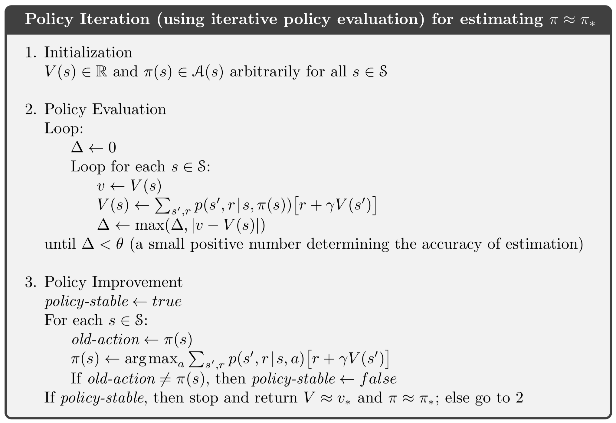
Homework: Modify codes given (or write code from scratch) to implement policy iteration for the grid world example 3.5 and compare your results to those in example 3.8 on page 65.

Chapter 4 Notes

Gridworld (Example 3.5) Solved by Policy Evaluation (Prediction) for v_\pi

Gridworld (Example 3.5) Solved by Policy Evaluation (Prediction) for q_\pi

Policy Improvement

Background

Goal

Deterministic Policies

Policy Improvement

Policy Improvement Theorem (Deterministic Policies)

Policy Iteration

$v_\pi$

$q_\pi$