Overview of MDPs

• Evaluative feedback
• Associative aspects
• Sequential decision making
• Tradeoff immediate vs. delayed rewards
• Bandits: \(q_\ast(a)\)
• MDPs: \(q_\ast(s,a)\) and \(v_\ast(s)\)

Agent-Environment Interface

Problem Representation

“Any problem of learning goal-directed behavior can be reduced to three signals passing back and forth between an agent and its environment.”

• Choices (actions of agent)
• Basis for choices (states of environment)
• Goal definition (rewards to agent)

Agent-Environment Interface

• Interaction at discrete time steps, \(t=0, 1, 2, 3, \cdots\)
• Agent: chooses actions \(A_t \in \mathcal{A}(s)\)
• Environment: has a state \(S_t\in \mathcal{S}\)
• Environment: generates rewards \(R_t \in \mathcal{R}\)
• Trajectory: \(S_0, A_0, R_1, S_1, A_1, R_2, S_2, A_2, R_3, S_3, \cdots\)

Time Steps

• \(t=0, 1, 2, 3, \cdots\)
• May refer to fixed intervals of real time
• May refer to arbitrary successive stages of decision making and acting

Actions

• \(A_t \in \mathcal{A}(s)\)
• Any decision we want to learn how to make
• Low-level controls - voltage on a motor (continuous)
• High-level decisions - have lunch (binary), go to graduate school (binary)
• Can be mental or computational (think about \(X\), focus on \(Y\))

States

• \(S_t\in \mathcal{S}\)
• Anything we can know that might be useful in decision making
• Low-level sensations (sensor readings)
• High-level and abstract (symbolic description of objects in a room)
• May include memory
• May be mental (not knowing: where are my keys)
• May be subjective (surprise in a clearly defined sense)

Rewards

• \(R_t \in \mathcal{R}\)
• Formalizes the goal of the agent
• Part of the environment
• Computed/derived inside natural or artificial (robotic) agents, but considered external to agent

Agent-Environment Boundary

• Environment: anything that cannot be changed arbitrarily by agent
• Boundary: limit of agent’s absolute control (but not of its knowledge)
• Robots: motors, linkages, sensors \(\in\) environment
• Person/animal: muscles, skeleton, sensory organs \(\in\) environment

Example: Bioreactor

• Objective: Determine temperature and stirring rate for bioreactor
• State: thermocouple, other sensors, ingredients, target chemicals
• Actions: target temperature and stirring rate (passed to lower level controller)
• Reward: rate of target chemical production
• States & actions: vectors
• Reward: scalar value

Example: Pick-and-Place Robot

• Objective: Control motion of robotic arm in repetitive task (fast smooth motion)
• State: Positions and velocities of linkages
• Action: Motor voltages
• Reward: +1 (for each pick-and-place success) - jerkiness of motion

Discuss these Examples

• Stop smoking
• Play Packman
• Invest wisely
• Driving to a destination (move the boundry around)

Look at Example 3.3

• Action set that depends on the state
• Markovity of states defined in graph
• Dynamics are tabulated (finite MDP)

Finite MDP

• \(\mathcal{S, A, R}\) are finite sets
• RVs \(S_t, A_t, R_t\) have PMFs
• MDP dynamics:

\[ \begin{gather} p(s',r | s, a) = \text{Pr}\left\{\begin{array}{c}S_t=s' \\ R_t=r\end{array} \bigg|\begin{array}{c} S_{t-1}=s \\ A_{t-1}=a\end{array}\right\} \\[1em] \sum_{s' \in \mathcal{S}} \sum_{r \in \mathcal{R}} p(s',r|s,a) = 1, \;\;\forall \;\; s\in \mathcal{S}, a\in \mathcal{A}(s) \end{gather} \]

Markov Property

• Not restriction on MDP
• Markovity is in the state

\[ (S_t,A_t) \mapsto S_{t+1} \]

Goals

• Maximize total amount of reward received
• Don’t focus on immediate (short run) reward
• Focus on cumulative reward in the long run

Rewards

• Incentivize what you want the agent to learn
• If you want the agent to learn “to do something for us, then provide rewards to it in such a way that in maximizing them the agent will also achieve our goals.”
• Rewards communicate what to achieve, not how to achieve it

Chess

• Reward winning (what)
• Don’t reward subgoals (how)
  • Taking opponent’s pieces (how)
  • Controlling center of board (how)
  • +10 for win (reward winning the game)
  • -1 for each turn (reward winning the game in few moves)

Examples

Do these reward the right thing?

• Robotic walking - make reward proportional to forward motion on each time step
• Escape maze - reward is -1 for every time step

Returns

• Choose \(A_t\) to maximize return \(G_t\)
• Return \(G_t\) is cumulative reward received after time \(t\)
• Return \(G_t = R_{t+1} + R_{t+2} + R_{t+3} + \cdots + R_T\)
• Return could be some other function of reward sequence
• Note: Action \(A_t\) cannot maximize \(G_{t-k}\) for \(k>0\)

Episodes

• Episode is a repeated interaction
  • Starting state is known or drawn from distribution
  • Ending in terminal state \(s\in \mathcal{S}^+\) at time \(T<\infty\)
  • \(T\) is an RV
• Episodic tasks (games, mazes, etc.)
• Nonepisodic tasks continue without end
  • Process control task
  • Robot with long life span
  • \(T=\infty\)

Discounting

• Choose \(A_t\) to maximize discounted return \(G_t = \sum_{k=0}^\infty \gamma^k R_{t+k+1}\)

• \(\gamma \in [0,1]\) is the discount rate

• Discounting puts diminishing weight on future rewards

• \(\gamma=0\) (myopic agent) focuses attention on immediate reward \(R_{t+1}\)

• \(\gamma \rightarrow 1\) (farsighted agent)

Recursion

\[ \begin{align} G_t &= \sum_{k=0}^\infty \gamma^k R_{t+k+1} = R_{t+1} + \gamma G_{t+1} \quad \forall \quad t<T \\ G_t &= \sum_{k=0}^\infty \gamma^k = \frac{1}{1-\gamma}, \quad R_t = 1 \quad \forall \quad t \end{align} \]

Example: Cart-Pole

Example: Cart-Pole

Maze escape robot

• \(R_t=1\) for esacpe and \(R_t=0\) otherwise. Why doesn’t this work?
• How can we communicate through the reward what we want the robot to do?

Task Types

• Episodic: \(S_{t,i}, A_{t,i}, R_{t,i}, \pi_{t,i}, T_i\) for the \(i^\text{th}\) episode
• Convention: Drop the \(i\) most of the time
• Continuing: \(S_{t}, A_{t}, R_{t}, \pi_{t}, T\)
• Same notation for both task types

Return

• Epsiodic: \(G_t = R_{t+1} + R_{t+2} + \cdots + R_{T}\)
• Continuing: \(G_t = R_{t+1} + R_{t+2} + R_{t+3} + \cdots\)
• Want same notation for both task types
• To unify notation, define absorbing (square) state for episodic task where rewards are zero

Unified Notation

\[ G_t = \sum_{k=0}^{T-t-1} \gamma^k R_{t+k+1} = \sum_{k=t+1}^T \gamma^{k-t-1} R_k \]

• Continuing: \(T=\infty\) and \(\gamma \in [0,1)\) (need convergence)
• Episodic: \(T<\infty\) and \(\gamma \in [0,1]\) (convergence guaranteed)
• Episode numbers not needed

Policy

\[ \begin{gather} \pi(a|s) = \text{Pr}\{A_t = a | S_t=s\} \\ a \in \mathcal{A}(s), \quad s \in \mathcal{S} \end{gather} \]

• Policy: How the agent chooses actions in the context of a state
• RL methods: How \(\pi\) changes based on experience

State-Value Function for Policy \(\pi\)

\[ v_\pi(s) = E_\pi[G_t | S_t=s] = E_\pi \left[\sum_{k=0}^{\infty} \gamma^k R_{t+k+1} \bigg| S_t=s\right] \]

• Expected return (value) when starting in state \(s\) and following policy \(\pi\) thereafter

Action-Value for Policy \(\pi\)

\[ \begin{align} q_\pi(s,a) &= E_\pi[G_t | S_t=s, A_t=a] \\ &= E_\pi\left[\sum_{k=0}^{\infty} \gamma^k R_{t+k+1} \bigg| S_t=s, A_t=a\right] \end{align} \]

• Expected return (value) of taking action \(a\) in state \(s\) and following policy \(\pi\) thereafter

Look Ahead (Monte Carlo Methods)

• Expectations in \(v_\pi\) and \(q_\pi\) can be estimated from sample averages over many episodes
• How? For each state maintain average return that followed that state under policy \(\pi\). This converges to \(v_\pi\).
• How? For each state-action pair maintain average return that followed under policy \(\pi\). This converges to \(q_\pi\).

Look Ahead (Approximation Methods)

• If too many states, then keeping averages in each state is not practical.
• Approximate \(v_\pi, q_\pi\) as parameterized functions (e.g. DNN) and adjust parameters to match observed returns.

Exercises

• Give an equation for \(v_\pi\) in terms of \(q_\pi\) and \(\pi\) (solution)
• Given an equation for \(q_\pi\) in terms of \(v_\pi\) and four-argument \(p\) (solution)

Answers

\[ \begin{align} v_\pi(s) &= \sum_a q_\pi(s,a) \pi (s|a)\\ q_\pi(s,a) &= \sum_{s'} \sum_r \left[ r + \gamma v_\pi(s') \right]p(s',r|s,a) \end{align} \]

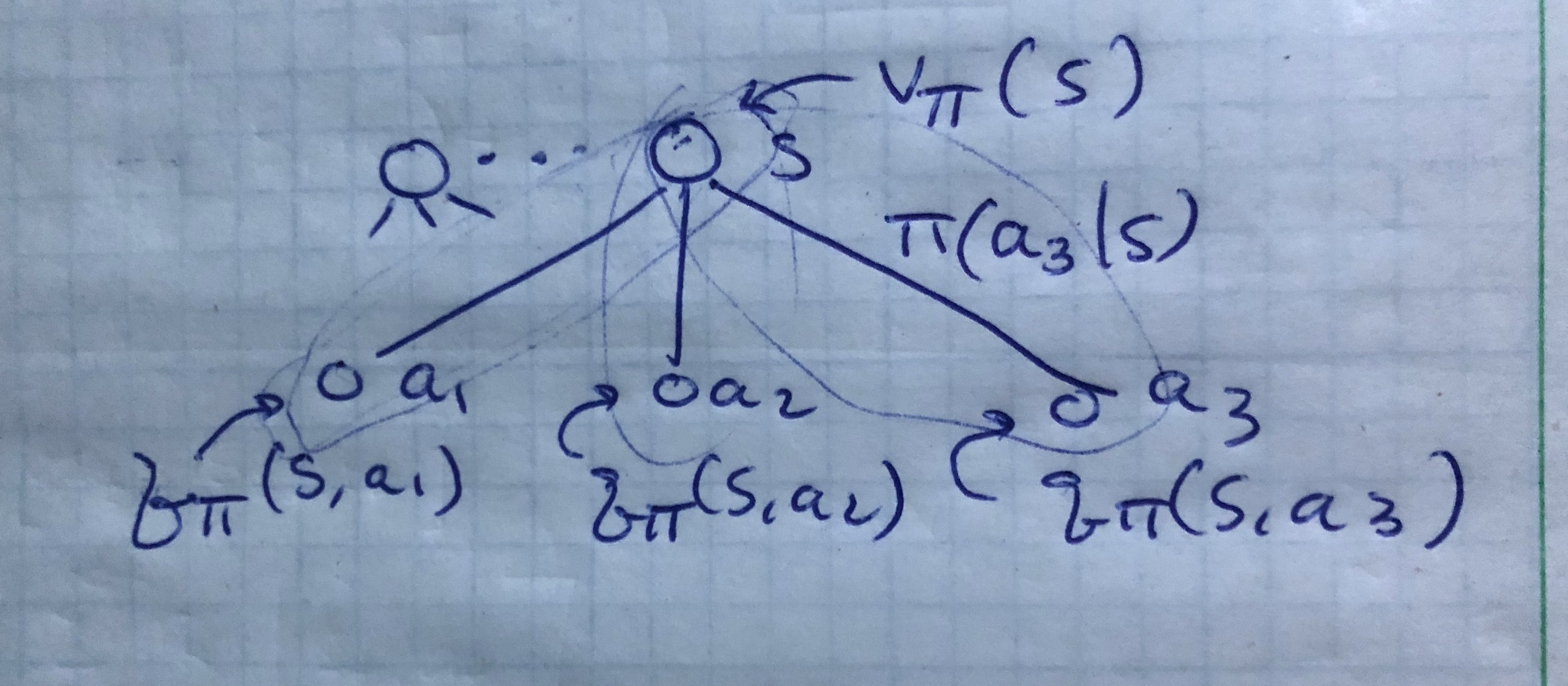
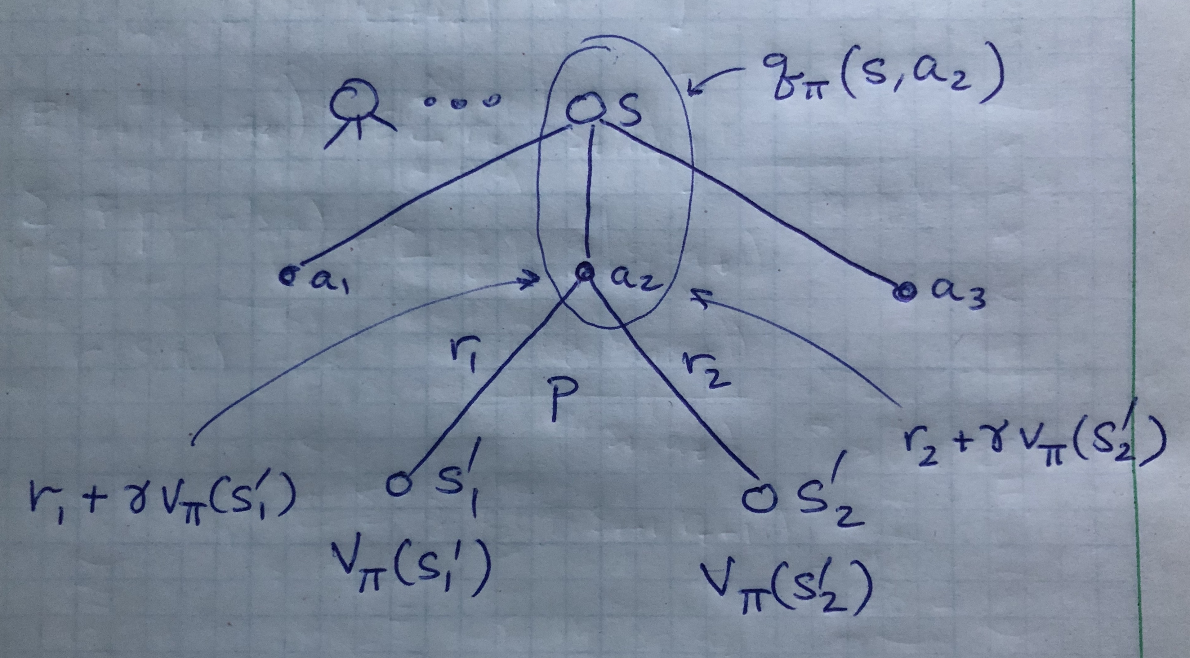
Backup Diagram for \(v_\pi\)

\[ v_\pi(s) = \sum_a q_\pi(s,a) \pi (s|a) \]

Backup Diagram for \(q_\pi\)

\[ q_\pi(s,a) = \sum_{s'} \sum_r \left[ r + \gamma v_\pi(s') \right]p(s',r|s,a) \]

Value Recursion

Substitute \(v_\pi\)-\(q_\pi\) relations into one another to obtain recursions.

\[ \begin{align} v_\pi(s) &= \sum_a \pi(a|s) \sum_{s',r} \left[ r + \gamma v_\pi(s') \right]p(s',r|s,a) \\ q_\pi(s,a) &= \sum_{s',r} \left[ r + \gamma \sum_{a'} q_\pi(s',a') \pi(s'|a') \right]p(s',r|s,a) \end{align} \]

State-Value Recursion

\[ v_\pi(s) = \sum_a \pi(a|s) \sum_{s',r} \left[ r + \gamma v_\pi(s') \right]p(s',r|s,a) \]

• Consistency condition between \(v_\pi(s)\) and \(v_\pi(s')\)
• Expected value of \(r+\gamma v_\pi(s')\) over \(p(s',r,a|s) = \pi(a|s)p(s',r|s,a)\)
• Bellman equation for \(v_\pi\)
• \(v_\pi\) is unique solution to Bellman equation
• Bellman equation: Compute, approximate, learn \(v_\pi\)

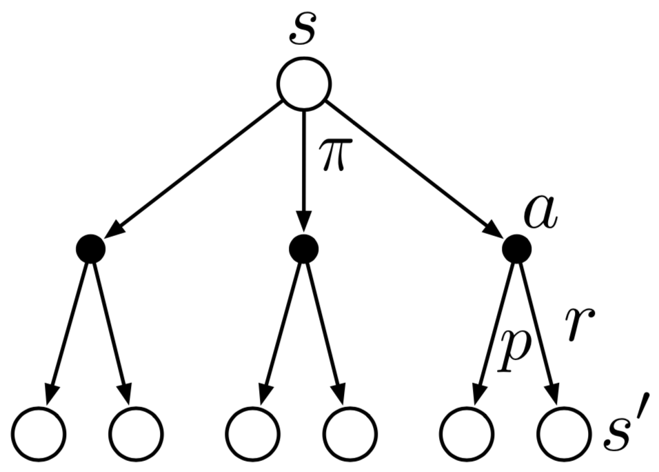
Backup Diagram for \(v_\pi\)

• Start state \(s\) at top (open circle)
• Policy \(\pi\) gives action \(a\) (solid circle)
• Environment responds with reward \(r\) and next state \(s'\) according to probability \(p\)

Gridworld

• See Example 3.5 in text (page 60).
• Here are my calculations.

Optimal Policies

• Value function defines a partial order for policies

\[ \pi \geq \pi' \quad \Leftrightarrow \quad v_\pi(s) \geq v_{\pi'}(s) \;\;\forall\;\;s \in \mathcal{S} \]

• An optimal policy exists but may not be unique
• Denote optimal policies by \(\pi_\ast\)
• Denote optimal state-value function \(v_\ast = v_{\pi_\ast}\)

Optimal Policies

\[ \begin{align} v_\ast(s) &= \max_\pi v_\pi(s) \;\;\forall\;\;s\in\mathcal{S} \\ q_\ast(s,a) &= \max_\pi q_\pi(s,a) \;\;\forall\;\;s\in\mathcal{S} \;\;\text{and}\;\; a\in\mathcal{A}(s) \end{align} \]

• The same policy optimizes both value functions

Relations

• Q: What does the optimal policy \(\pi_\ast\) look like?
• A: It puts all its weight on the best action (greed)

\[ \begin{gather} \pi_\ast(a|s) = \mathbb{1}_{a=a_\ast} = \begin{cases} 1, & a=a_\ast \\ 0, & \text{otherwise} \end{cases} \\[1em] v_\ast(s) = \sum_{a\in\mathcal{A}(s)} \pi_\ast(a|s) q_\ast(s,a) = \max_{a\in\mathcal{A}(s)} q_\ast(s,a) \end{gather} \]

Recursion for Optimal Value Function

Leveraging this derivation and \(\pi=\pi_\ast\), we have

\[ \begin{align} v_\ast(s) &= \max_a q_\ast(s,a) \\ &= \max_a E[R_{t+1} + \gamma G_{t+1} | S_t=s,A_t=a] \\ &= \max_a E[R_{t+1} + \gamma v_\ast(S_{t+1}) | S_t=s, A_t=a] \\ &= \max_a \sum_{s',r} p(s',r|s,a) [r + \gamma v_\ast(s')] \end{align} \]

Apply Greed

\[ \begin{align} v_\pi(s) &= \sum_a \pi(a|s) \sum_{s',r} \left[ r + \gamma v_\pi(s') \right]p(s',r|s,a) \\ v_\ast(s) &= \max_a \sum_{s',r} \left[ r + \gamma v_\ast(s') \right]p(s',r|s,a) \end{align} \]

\[ \sum_a \pi_\ast(a|s) \quad \overset{\text{greed}}{\longrightarrow} \quad \max_a \]

Recursion for Optimal Action-Value Function

Applying greed, we have

\[ \begin{align} q_\pi(s,a) &= \sum_{s',r} p(s',r|s,a) \left[ r + \gamma \sum_{a'} \pi(s'|a') q_\pi(s',a') \right] \\ q_\ast(s,a) &= \sum_{s',r} p(s',r|s,a)\left[ r + \gamma \max_{a'} q_\ast(s',a') \right] \end{align} \]

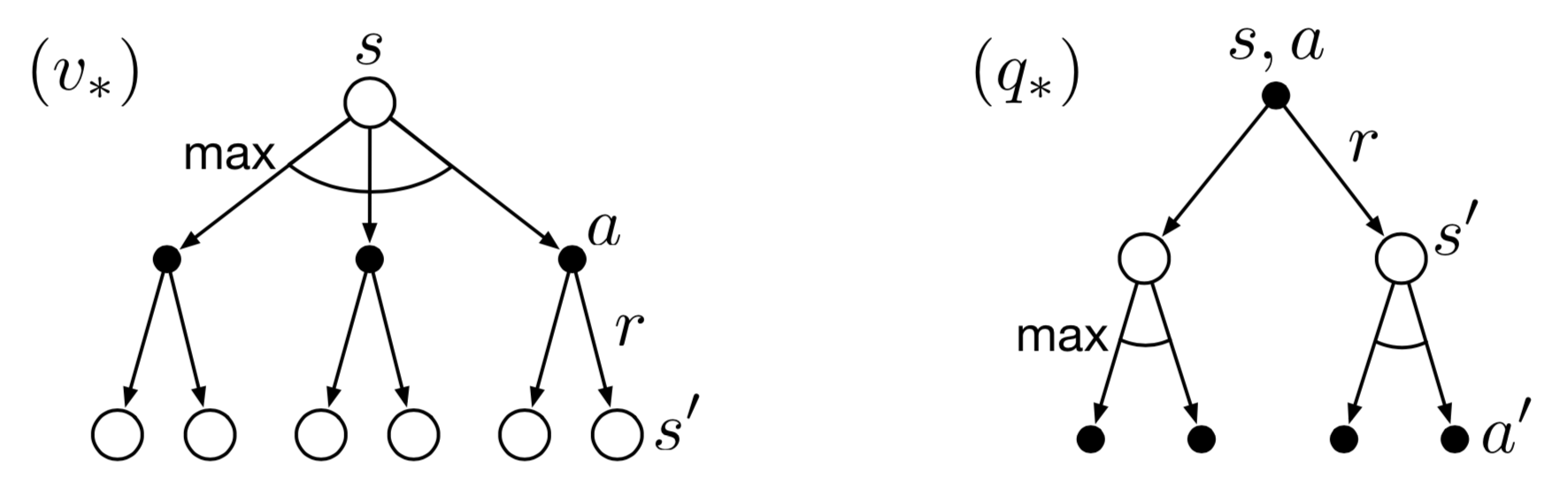
Backup Diagrams for Optimal Value Functions

Optimal Policy for Gridworld

(We don’t yet know how to find \(v_\ast\). Take this as given for now.)

Optimal Policy \(\leftarrow\) Optimal Value

• Given \(v_\ast(s)\), \(\pi_\ast(a|s)\) assigns non-zero probability to best action(s) and zero probability to all other actions
• Optimal policy \(\pi_\ast\) is greedy wrt optimal value \(v_\ast\)
• A one-step (short-run) search is long-run optimal
• \(v_\ast\) “takes into account the reward consequences of all possible future behavior”
• Expected long-term return is encoded into \(v_\ast\)

Optimal Policy \(\leftarrow\) Optimal Value

• Same for \(q_\ast(s,a)\) … in any state \(s\), choose the best action \(a\)
• Costs more to store \(q_\ast(s,a)\) than \(v_\ast(s)\)
• \(q_\ast\) encodes best action(s) without needing to know values of next states or environment dynamics \(p(s',r|s,a)\)

Bellman’s Eqations in Practice

\[ \begin{align} v_\ast(s) &= \max_a \sum_{s',r} \left[ r + \gamma v_\ast(s') \right]p(s',r|s,a) \\ q_\ast(s,a) &= \sum_{s',r} p(s',r|s,a)\left[ r + \gamma \max_{a'} q_\ast(s',a') \right] \end{align} \]

• Usually don’t know \(p(s',r|s,a)\)
• Usually can’t compute (sum and max too big)
• Markov property (assume this)