Background

• Past: Learned \(\hat{v}(s,\mathbf{w})\) or \(\hat{q}(s,a,\mathbf{w})\)
• Past: Policy was inferred from value function
• New: Learn parameterized policy \(\pi(a|s,\mathbf{\theta}) = \text{Pr}\{A_t=a|S_t=s,\mathbf{\theta}_t = \mathbf{\theta}\}\)
• Value functions may still be used to learn policy parameter

\[ \begin{gather} \mathbf{\theta} \in \mathbb{R}^{d'} \qquad (\text{policy parameter}) \\ \mathbf{w} \in \mathbb{R}^{d} \qquad (\text{value parameter}) \end{gather} \]

Policy Gradient Methods

• Update \(\mathbf{\theta}\) to maximize performance measure \(J(\mathbf{\theta})\)
• Gradient ascent:

\[ \mathbf{\theta}_{t+1} = \mathbf{\theta}_{t} + \alpha \widehat{\nabla J(\mathbf{\theta})} \]

where \(\widehat{\nabla J(\mathbf{\theta})}\) is a stochastic estimate in which

\[ E\{\widehat{\nabla J(\mathbf{\theta})}\} \approx \nabla J(\mathbf{\theta}) \]

Actor-Critic Methods

• Policy gradient methods: SGA on \(J(\mathbf{\theta})\) whether or not a value function is also learned
• Actor-critic methods: Learn both policy (actor) and value (critic) approximations

Exploration vs. Exploitation

• To ensure exploration, require non-deterministic policy \(\pi(a|s,\mathbf{\theta}) \in (0,1)\)
• PG good for continuous action spaces
• Parameterized preferences \(h(s,a,\mathbf{\theta})\)
• Soft-max policy distribution

\[ \pi(a|s,\mathbf{\theta}) = \frac{e^{h(s,a,\mathbf{\theta})}}{\sum_b e^{h(s,b,\mathbf{\theta})}} \]

“soft-max in action preferences”

Parameterizations

• \(h(s,a,\mathbf{\theta})\) could be a DNN (as in AlphaGo)
• \(h(s,a,\mathbf{\theta}) = \mathbf{\theta}^T \mathbf{x}(s,a)\) or linear in features

Advantages of Policy Approx.

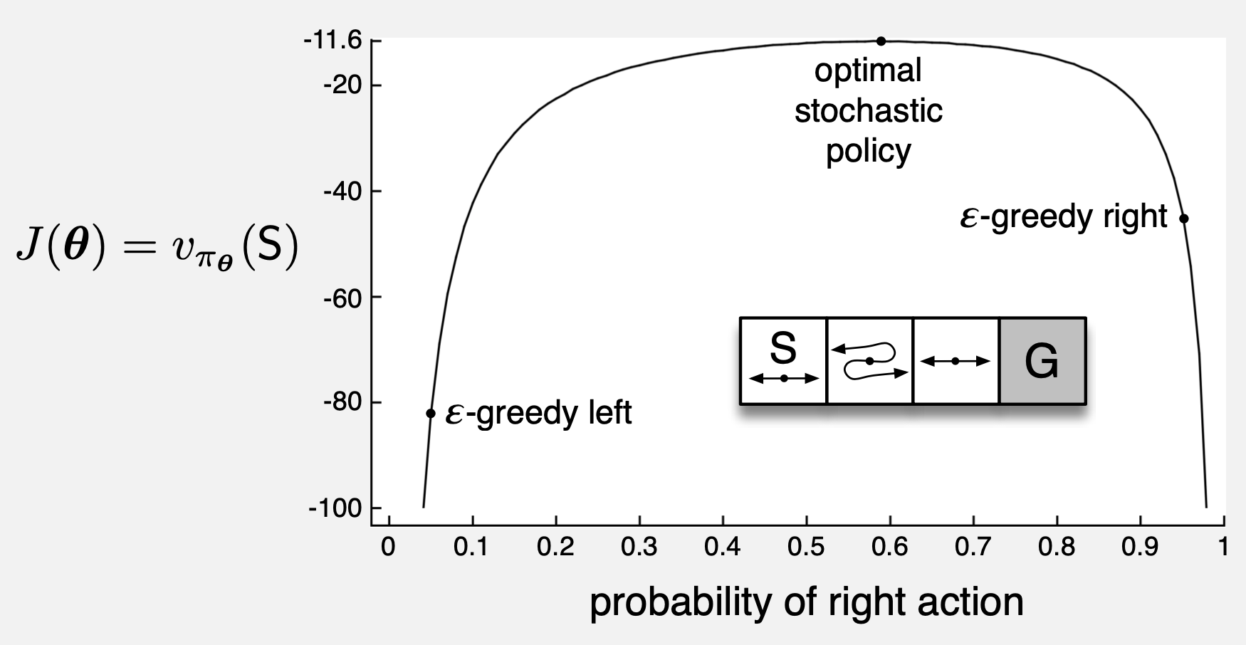
• \(\varepsilon\)-greed action selection leaves \(\varepsilon\) probability of random action
• Parameterized policy can approach a deterministic (optimal) policy to the extent allowed by the parameterization
• “Action-value methods have no natural way of finding stochast optimal policies…”
• “…whereas policy approximation methods can.”

Example 13.1 (page 323)

More Advantages

• The policy function may be a simpler function to approximate
• For some the action-value function is simpler and for others the policy function is simplier
• If policy is simpler, then PG will learn faster and yield superior asymptotic policy
• Policy methods offer good way to inject prior knowledge about form of policy into RL

Even More Advantages

• Policy approx.: Action probabilities change smoothly as function of \(\mathbf{\theta}\)
• Value approx.: Action values (\(\hat{v}\) and \(\hat{q}\)) change smoothly as a function of \(\mathbf{w}\), but \(\varepsilon\)-greedy policy may change dramatically for small change in value if that change results in a different action haveing maximal value
• Stronger convergence guarantees for PG

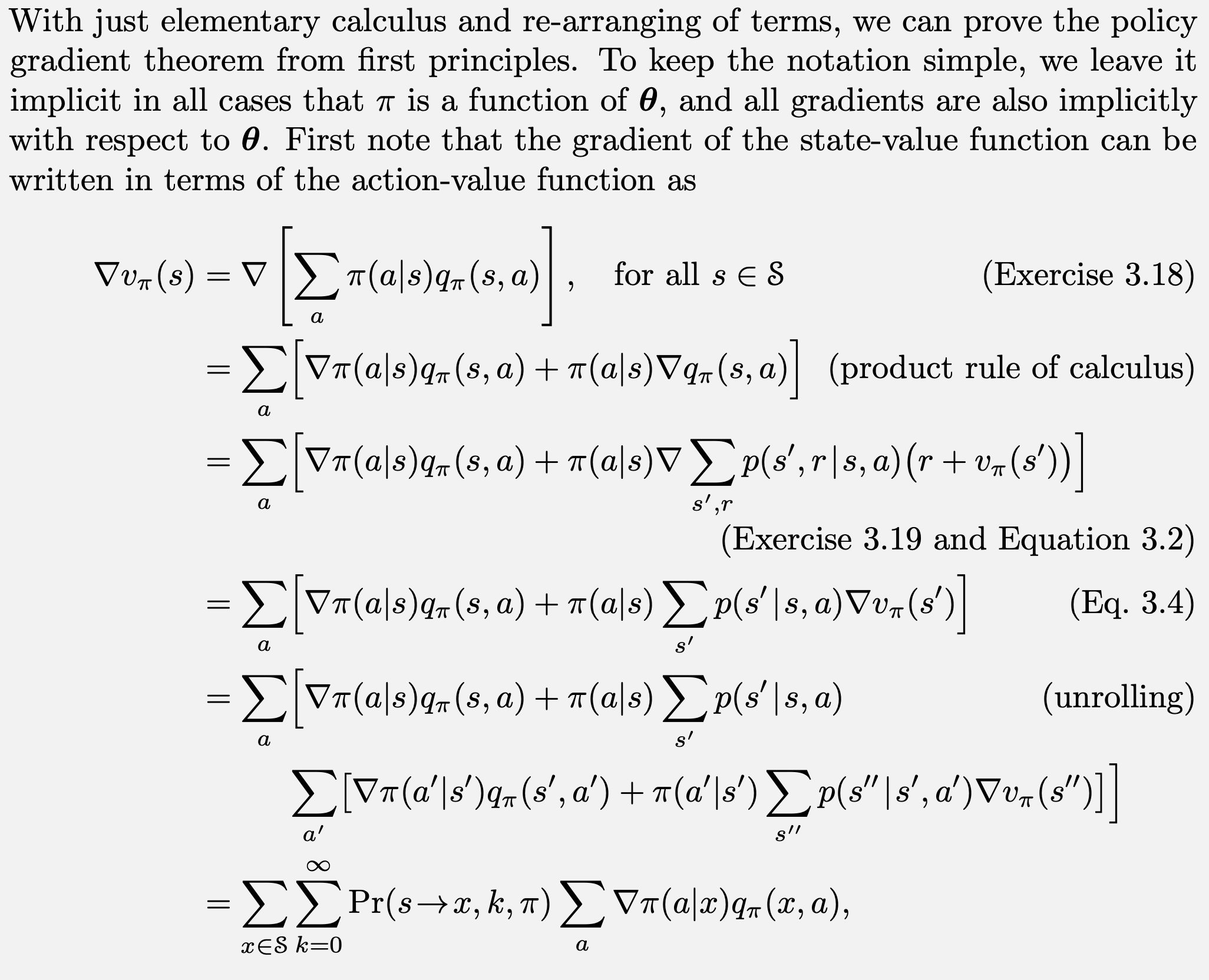
Policy Gradient Theorem

• In the episodic case: \(J(\mathbf{\theta}) = v_{\pi_\mathbf{\theta}}(s_0)\)
• Depends on:
  • 1. Action selections (depends on \(\mathbf{\theta}\))
  • 2. State distribution (depends on \(\mathbf{\theta}\))
• 1. is straightforward to deal with: \((\mathbf{\theta},s_0) \rightarrow \text{actions}\)
• 2. is hard because it depends on the environment which is unknown
• How can we estimate \(\widehat{\nabla J(\mathbf{\theta})}\)?

Policy Gradient Theorem

\[ \nabla J(\mathbf{\theta}) = C\cdot \sum_s \mu(s) \sum_a q_\pi(s,a) \nabla \pi(a|s,\mathbf{\theta}) \]

All-Actions

\[ \begin{align} \nabla J(\mathbf{\theta}) &\propto \sum_s \mu(s) \sum_a q_\pi(s,a) \nabla \pi(a|s,\mathbf{\theta})\\ &= E\left[ \sum_a q_\pi(S_t,a)\nabla\pi(a|S_t,\mathbf{\theta})\right] \\ \mathbf{\theta}_{t+1} &= \mathbf{\theta} +\alpha \sum_a \hat{q}(S_t,a,\mathbf{w}) \nabla \pi(a,|S_t,\mathbf{\theta}) \end{align} \]

• Involves all actions (even ones not taken)

REINFORCE

\[ \begin{align} \nabla J(\mathbf{\theta}) &= E\left[ \sum_a q_\pi(S_t,a)\nabla\pi(a|S_t,\mathbf{\theta})\right] \\ &= E\left[ \sum_a \pi(a|S_t,\mathbf{\theta}) q_\pi(S_t,a)\frac{\nabla\pi(a|S_t,\mathbf{\theta})}{\pi(a|S_t,\mathbf{\theta})}\right] \\ &= E\left[ q_\pi(S_t,A_t)\frac{\nabla\pi(A_t|S_t,\mathbf{\theta})}{\pi(A_t|S_t,\mathbf{\theta})}\right] \end{align} \]

REINFORCE

\[ \begin{align} \nabla J(\mathbf{\theta}) &= E\left[ q_\pi(S_t,A_t)\frac{\nabla\pi(A_t|S_t,\mathbf{\theta})}{\pi(A_t|S_t,\mathbf{\theta})}\right] \\ &= E\left[ G_t\frac{\nabla\pi(A_t|S_t,\mathbf{\theta})}{\pi(A_t|S_t,\mathbf{\theta})}\right] \end{align} \]

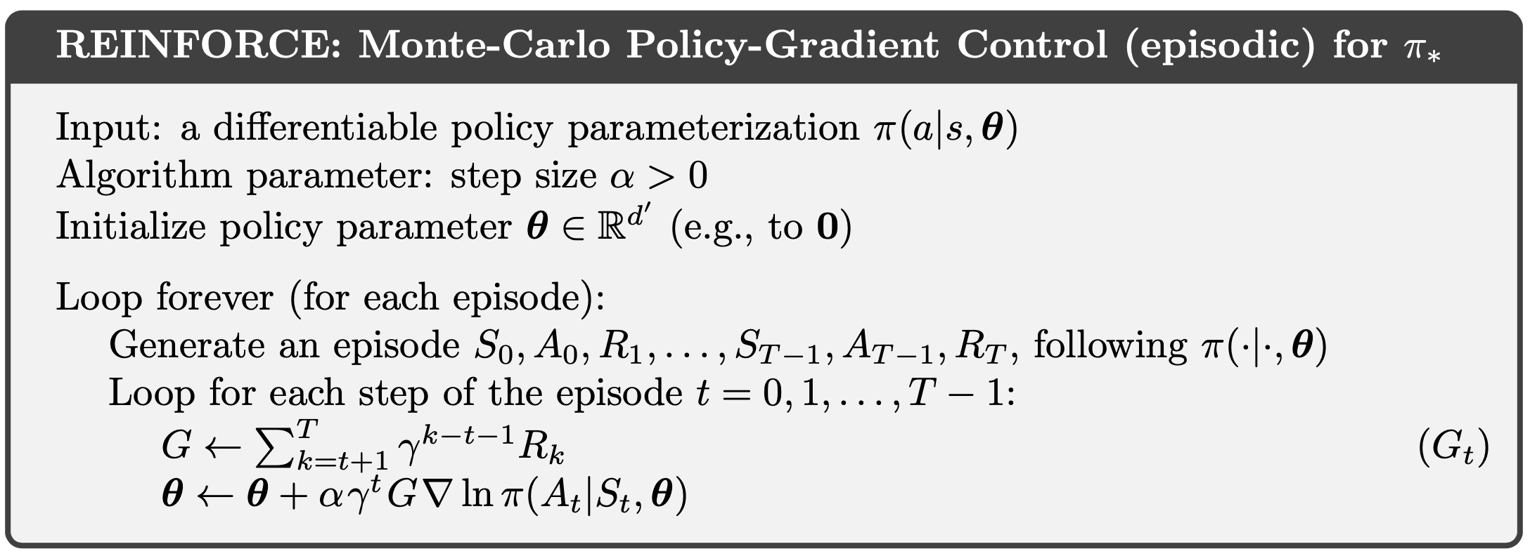
REINFORCE Update

\[ \mathbf{\theta}_{t+1} = \mathbf{\theta} +\alpha G_t\frac{\nabla\pi(A_t|S_t,\mathbf{\theta})}{\pi(A_t|S_t,\mathbf{\theta})} \]

• Increases prob. of repeating \(A_t\) on future visits to \(S_t\)
• Favors actions that yield higher returns due to product with \(G_t\)
• \(\pi\) in denom. removes advantage of frequently selected actions

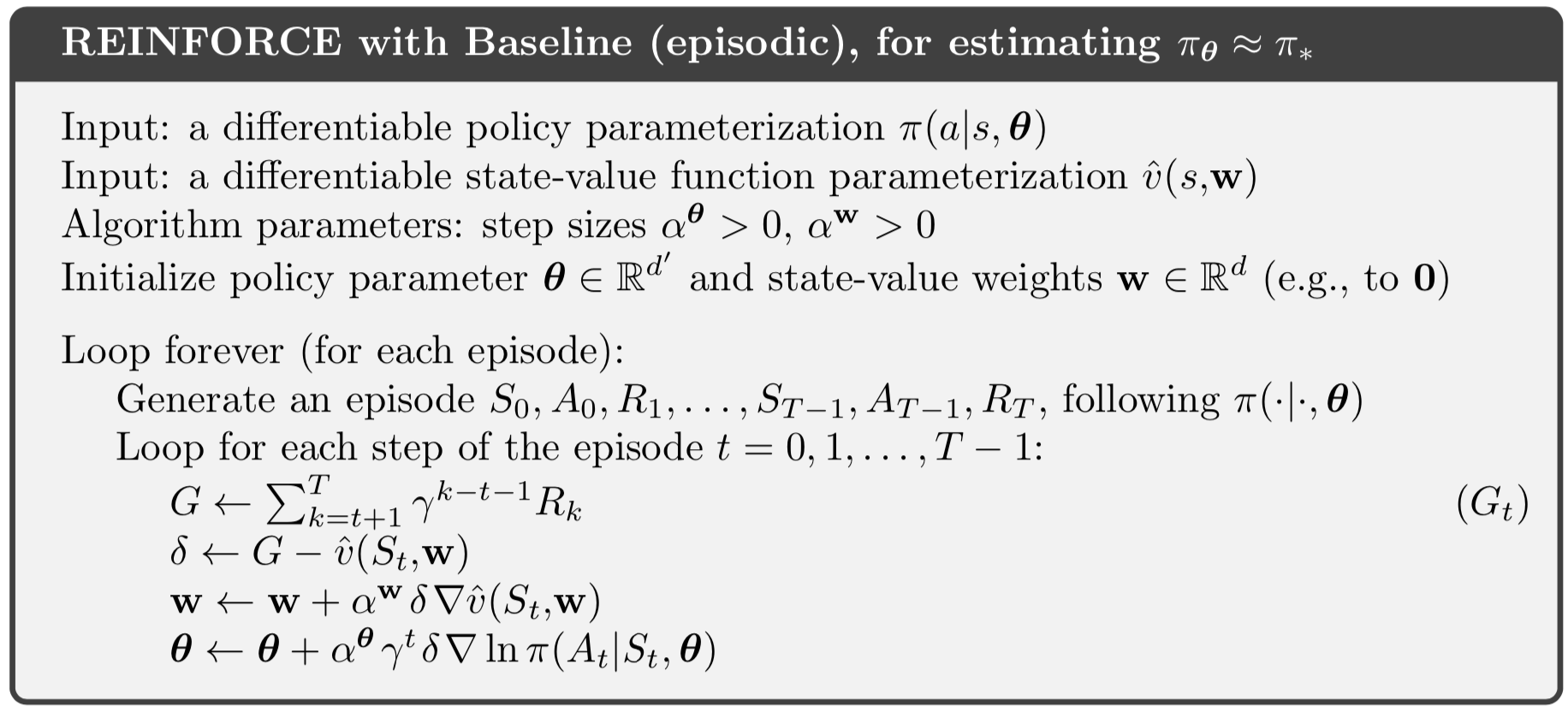
REINFORCE Algorithm

REINFORCE Example

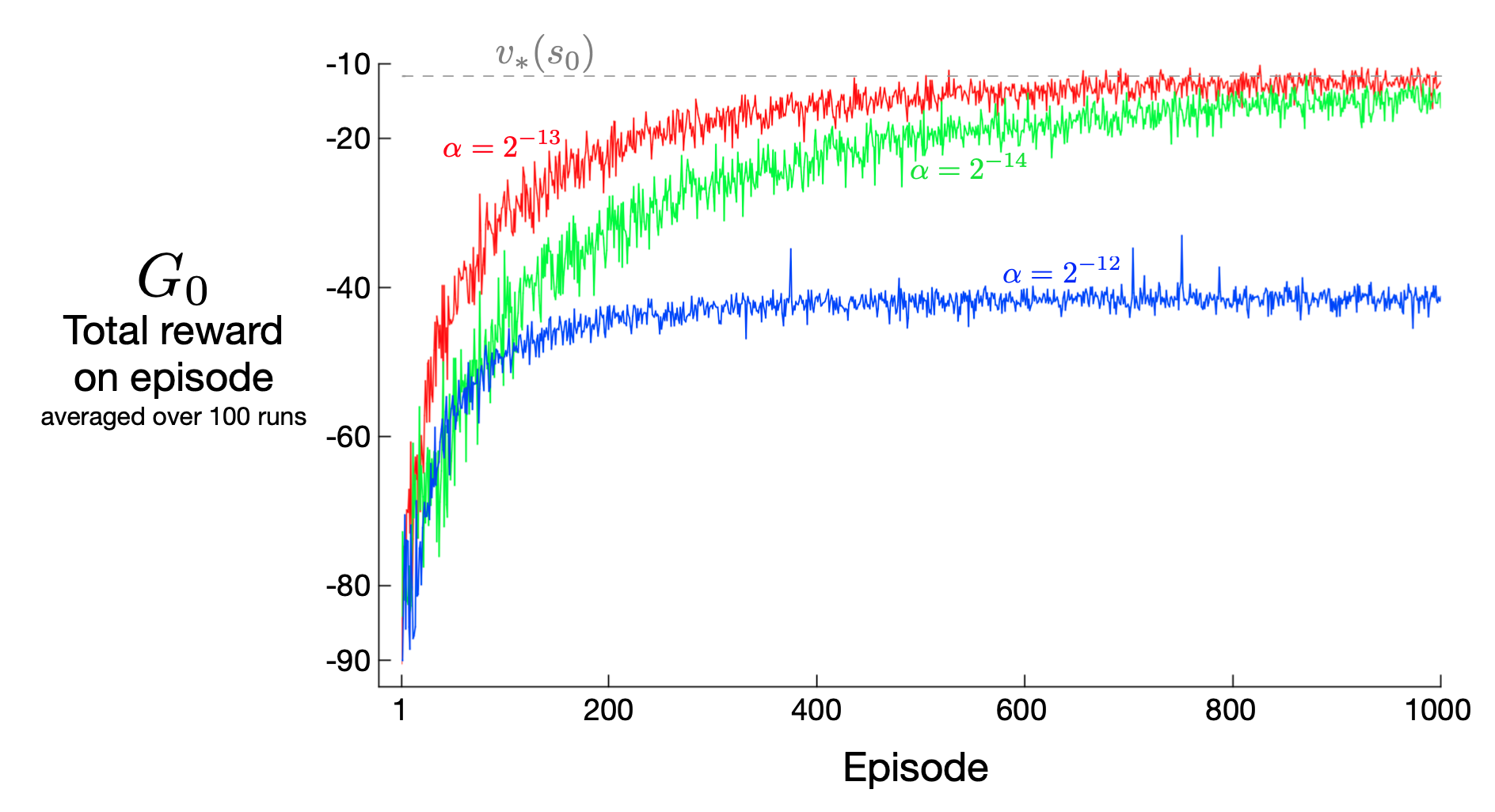
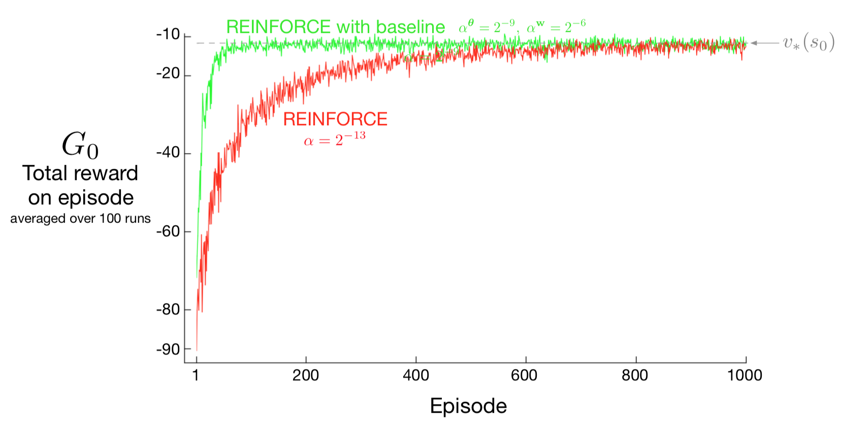
REINFORCE Performance

• High variance \(\rightarrow\) slow learning

Background

Policy Gradient Theorem

\[ \nabla J(\mathbf{\theta}) = C\cdot \sum_s \mu(s) \sum_a q_\pi(s,a) \nabla \pi(a|s,\mathbf{\theta}) \]

Policy Gradient with Baseline Theorem

\[ \nabla J(\mathbf{\theta}) = C\cdot \sum_s \mu(s) \sum_a \left(q_\pi(s,a)-b(s)\right) \nabla \pi(a|s,\mathbf{\theta}) \]

Proof

\[ \begin{align} \sum_a b(s) \nabla \pi(a|s,\mathbf{\theta}) &= b(s) \nabla \sum_a \pi(a|s,\mathbf{\theta}) \\ & = b(s) \nabla 1 = 0 \end{align} \]

Subtracting a baseline does nothing to the gradient

\[ \nabla J(\mathbf{\theta}) = C\cdot \sum_s \mu(s) \sum_a \left(q_\pi(s,a)-b(s)\right) \nabla \pi(a|s,\mathbf{\theta}) \]

REINFORCE with Baseline

\[ \mathbf{\theta}_{t+1} = \mathbf{\theta} +\alpha \left(G_t-b(S_t)\right)\frac{\nabla\pi(A_t|S_t,\mathbf{\theta})}{\pi(A_t|S_t,\mathbf{\theta})} \]

• Baseline does not change expectted value
• Baseline can reduce variance (speed learning)
• Could use \(b(s) = \hat{v}(s,\mathbf{w})\)

REINFORCE with Baseline

Performance

Comments

• Actor-Critic (AC): Approximate policy and value
• REINFORCE with baseline: Learns approximate policy and value but is not AC
• Why? Becuase approximated value is used as baseline, not as a critic
• REINFORCE with Basesline is unbiased and converges asymptotically
• REINFORCE can be slow due to high variance
• Baseline reduces variance and accelerates learning

Critic

• Approximated value function
• Approx. value function used for bootstrapping
• Updating the approx. value for \(s\) from approx. value for \(s'\)
• Bootstrapping \(\rightarrow\) bias & asymptotic dependence on quality of approximation

Actor-Critic Methods

• REINFORCE is Monte Carlo method
  • Pro: unbaised
  • Con: high variance, slow convergence, episodic
• Actor-Critic
  • Temporal difference: online, fast convergence, continuing
  • Multi-step methods: choose degree of bootstrapping

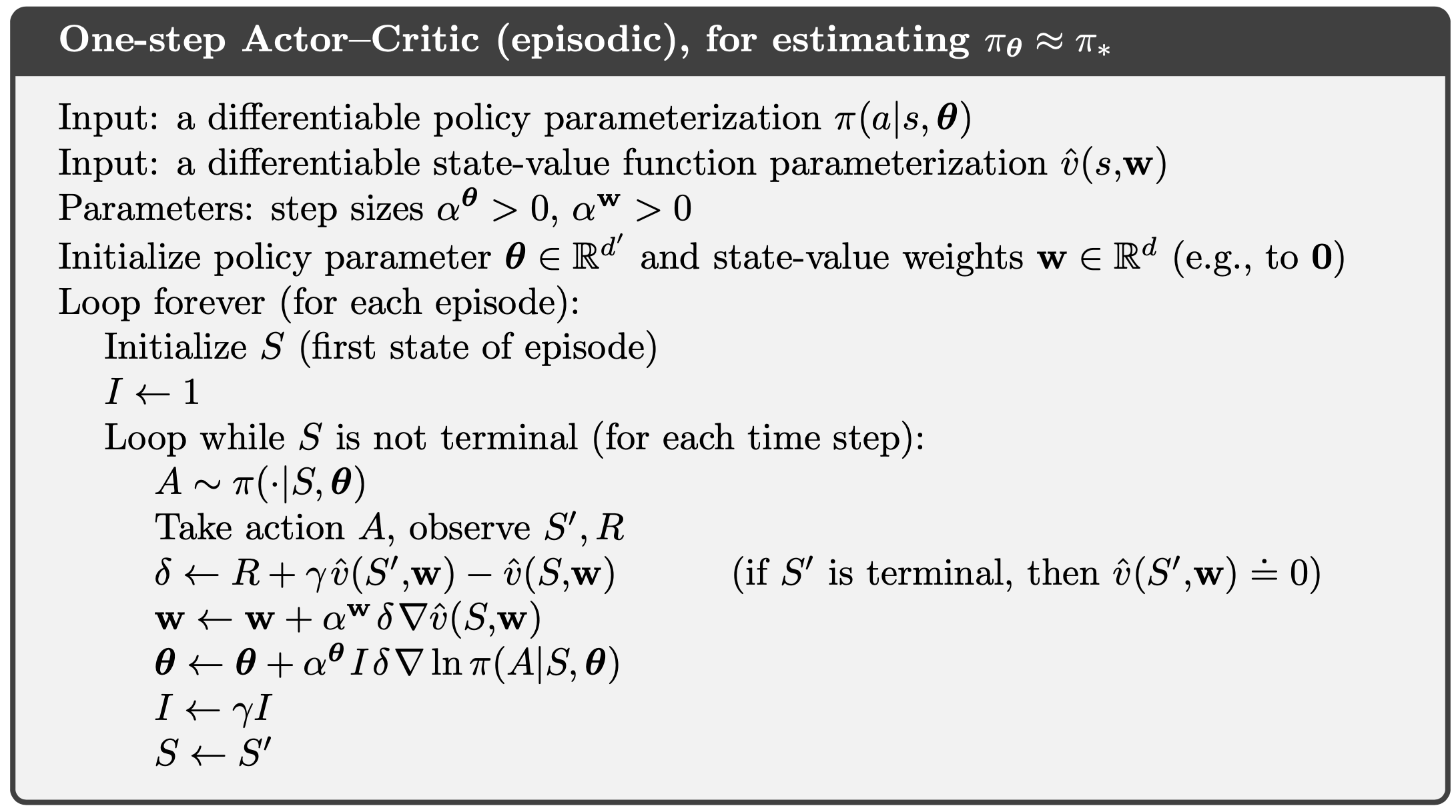
One-Step Actor-Critic

• Analog of TD(0), Sarsa(0), Q-learning
• Online, incremental, avoid eligibility traces
• Replace full return in REINFORCE with Baseline with one-step return and \(\hat{v}\) as baseline

(see equations on next page)

AC Update

\[ \begin{align} \mathbf{\theta}_{t+1} &= \mathbf{\theta}_t + \alpha \left( G_{t:t+1} -\hat{v}(S_t,\mathbf{w}) \right) \frac{\nabla \pi(A_t|S_t,\mathbf{\theta}_t)}{\pi(A_t|S_t,\mathbf{\theta}_t)} \\ &= \mathbf{\theta}_t + \alpha \left( R_{t+1} + \gamma \hat{v}(S_{t+1},\mathbf{w}) -\hat{v}(S_t,\mathbf{w}) \right) \frac{\nabla \pi(A_t|S_t,\mathbf{\theta}_t)}{\pi(A_t|S_t,\mathbf{\theta}_t)} \\ &= \mathbf{\theta}_t + \alpha \delta_t \frac{\nabla \pi(A_t|S_t,\mathbf{\theta}_t)}{\pi(A_t|S_t,\mathbf{\theta}_t)} \end{align} \]

One-Step AC Control

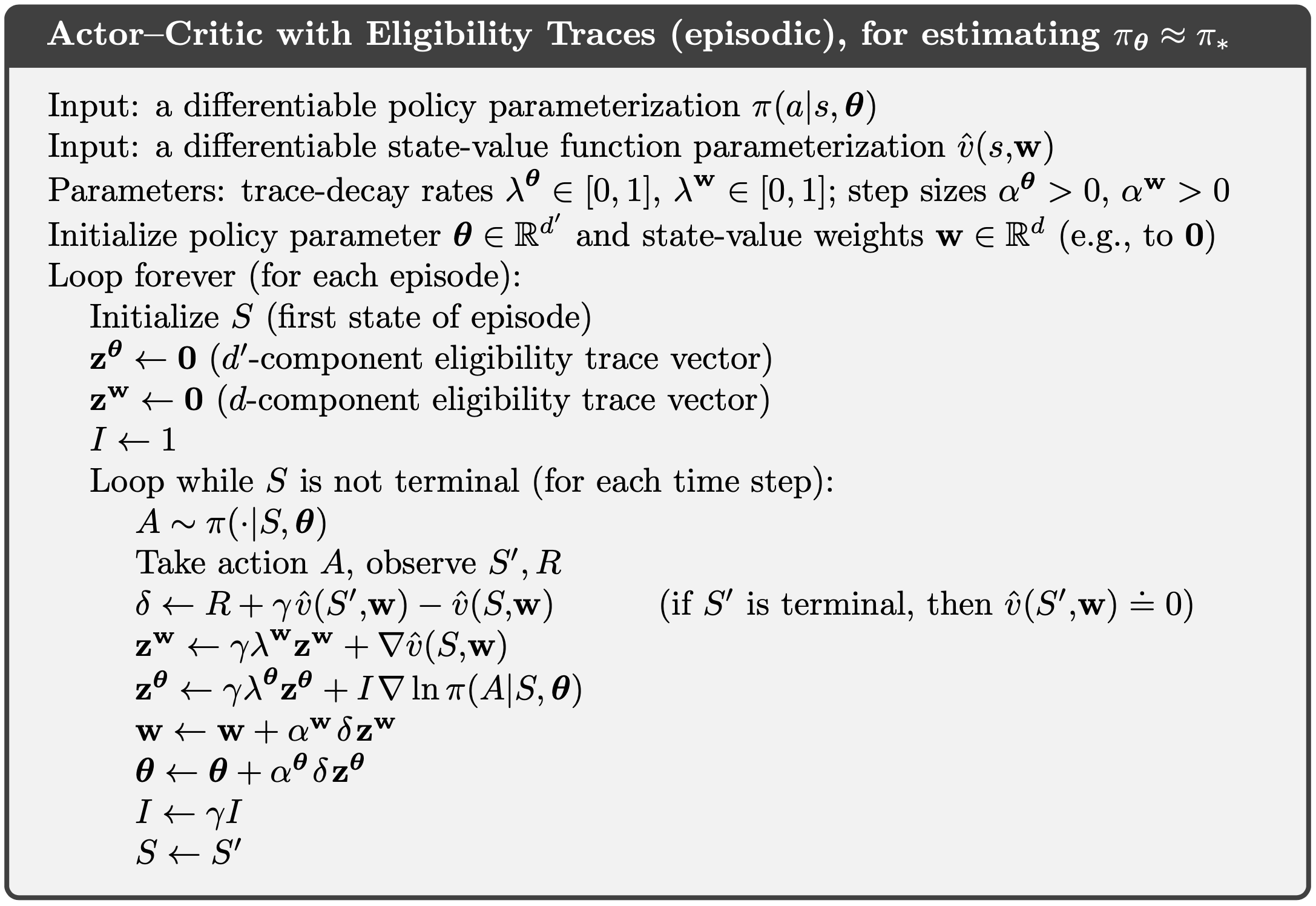
AC Control with Eligibility Traces

Policy Gradient for Continuing Problems

• Average rate of reward per time step \(r(\pi)\) (from chapter 10)
• Differential return \(G_t = R_{t+1} - r(\pi) + R_{t+2} - r(\pi) + \cdots\)
• Policy Gradient Theorem can be exteded to continuing case
• See book

Background

• Till now “everything” assumed discrete & finite action spaces
• Policy \(\pi(a|s,\mathbf{\theta})\) had soft-max output “layer”
• To take action:
  • Calculate probability \(\pi(a|s,\mathbf{\theta})\) for each \(a\in \mathcal{A}\)
  • Draw random action from this distribution
• Q: What to do for large discrete or continuous action spaces?
• A: Learn statistics/parameters of the distribution

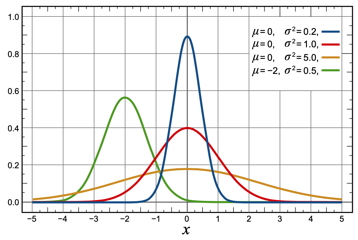
Gaussian Policy

\[ \begin{gather} \pi(a|s,\mathbf{\theta}) = \frac{1}{\sigma(s,\mathbf{\theta})\sqrt{2\pi}} \exp\left(-\frac{(a-\mu(s,\mathbf{\theta}))^2}{2\sigma(s,\mathbf{\theta})^2}\right) \\ \mu(s,\mathbf{\theta}) = \mathbf{\theta}_\mu^T \mathbf{x}_\mu(s) \qquad \sigma(s,\mathbf{\theta}) = \exp(\mathbf{\theta}_\sigma)^T \mathbf{x}_\sigma(s) \end{gather} \]