Maximum Margin Classifier
Suppose we are given samples from two different classes, where is the class label. The classification problem is to find a function that agrees with the class labels, for all . Here we consider only affine functions . A classifier is a pair such that .
Derivation
Given a vector and samples and on the margins, we have
Subtracting yields
which will be used later.
The width of the slab may be computed as the length of the projected difference of and onto ,
The margin is half of the slab width
Thus, maximizing the margin is equivalent to minimizing . The maximum margin classifier may be obtained by solving
When the samples are not separable by a hyperplane, we may introduce non-negative variables to relax the constraints
We want to minimize the extent to which the original constraints are violated. This leads to the modified problem
A closely related problem is
Show that the dual of the first problem is given by
and the dual of the second problem is given by
In both cases show that the optimal is a weighted linear combination of the data ,
Substituting this expression for into gives the classification function
Kernel Functions
Notice that everywhere that a test vector or training vector appears in the dual objective function or in the classification function, it appears as an inner product. Skipping a lot of background material, it is common to replace the inner product by the kerlnel function . Popular kernels for classification include the following examples.
The evaluation of many kernel functions is equivalent to promoting to a higher dimension through a nonlinear mapping, and then evaluating the inner product in that higher dimensional space. This is advantageous becuase data that is not separable in its native format may be linearly separable in a higher dimensional space.
Substituting the kernel function into the objective function leads to the following optimization problem.
or
where and is the matrix with entries .
It also leads to the classifier
Barrier Method
Using the barrier method, the inequality constraints can be incorporated into the objective function as follows,
The Lagrangian for this problem is
The KKT equations are as follows:
Newton's Method
Using the first order Taylor approximation for the inverse function
substitution into the KKT equations and linearize to obtain
Rewrite these quations in matrix-vector form to obtain,
where the assumption that are primal feasible was used. A feasible point must satisfy
This can be achieved by observing the following,
provided
Observing that and , define
and set
then is primal feasible. Of course other initializations are possible. It's a big feasible set!
Algorithm
blah, blah, blah ...
Block Gaussian Elimination
blah, blah, blah ...
Assignment
Do the following:
- Write code to solve the quadratic program (QP) above with inequality and equality constraints.
- Use the linear kernel and demonstrate 100% correct classification on the linearly separable dataset. Use plots to show the dataset, the classifer function, the margins, and the support vectors.
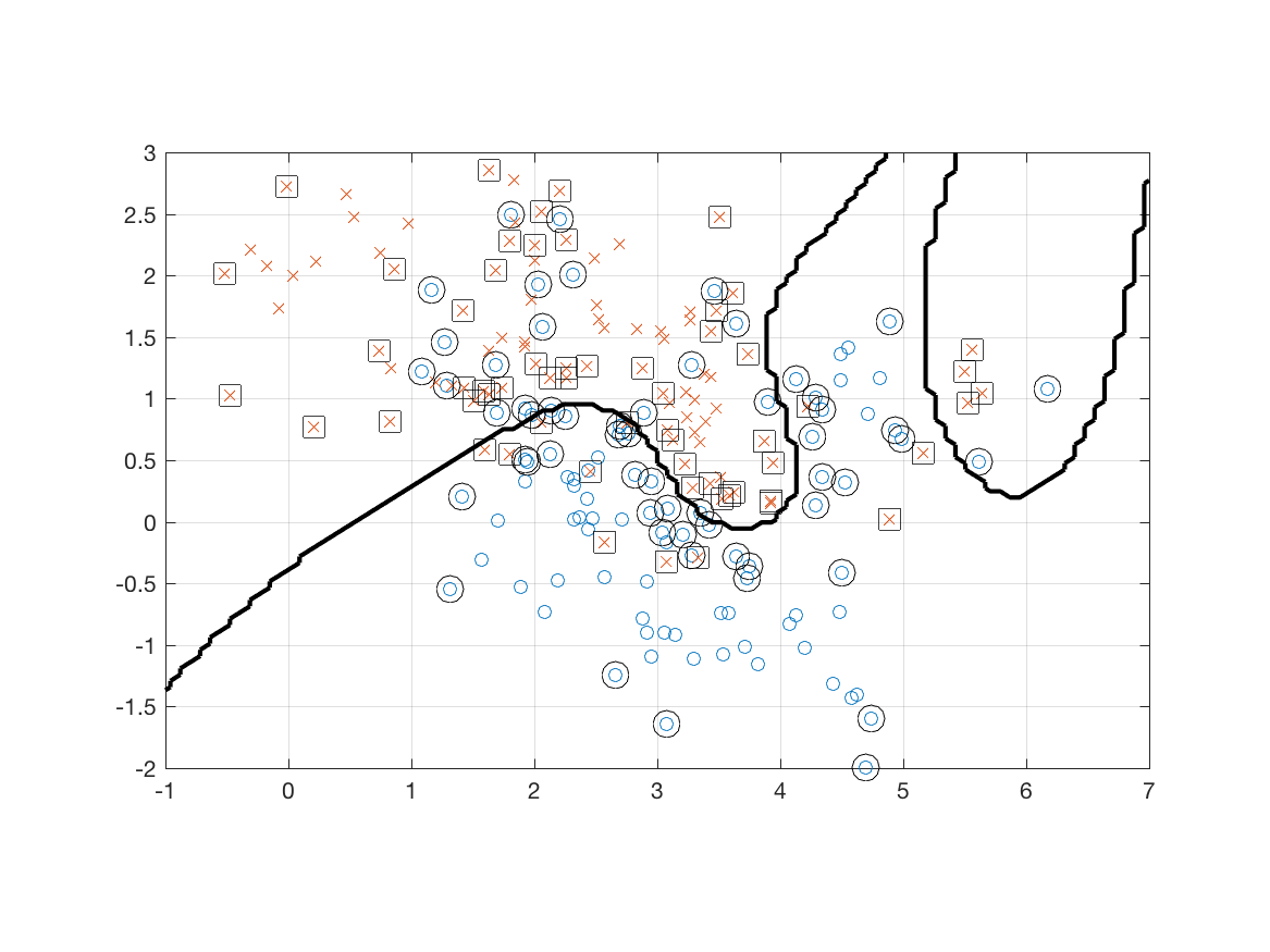
- Use the linear kernel on the mixture dataset. Use plots to show the dataset, the classifer function, the margins, and the support vectors. What is the classification error rate on the training dataset?
- Use the radial basis function kernel on the mixture dataset. Use plots to show the dataset, the classifer function, the margins, and the support vectors. What is the classification error rate on the training dataset?
- Use the linear kernel on the digits dataset. (Only classify digits "0" and "1".) Are the training data linearly separable. What is the classification error rate on the training and test sets?
- Use the radial basis function kernel on the digits dataset. Are the training data separable in this case? What is the classification error rate on the training and test sets?
Datasets
- Linearly separable data (two-dimensional data). Dataset1, dataset2.
- Mixture data (two-dimensional data) (from The Elements of Statistical Learning) Mixture set.
- Digits (256-dimensional data) (from The Elements of Statistical Learning) Train, test.
Note: Tables of data in text files can be loaded into Matlab using the command a = textread('train.txt');, for example. In the digits data, the file format is as follows. Each row corresponds to a digit. The first element is the digit, an integer between 0 and 9, inclusive. The next 256 elements are the grayscale pixel values in a 16 x 16 image of the digit in row scanned order.
xxxxxxxxxxa = textread('train.txt'); % Load the digits database from file.[num_digits,nc] = size(a); % How many digits are in the database?i = 200; % Select an image to view.d = a(i,1); % Get the digit.p = reshape(a(i,1+[1:256]),16,16).'; % Reshape the pixel data to an image.imagesc(p); axis image; shg; % Show an image of the digit.disp(sum(a(:,1)==0)); % How many zeros are there in the database?disp(sum(a(:,1)==5)); % How many fives are in the database?% And so on...Results
For the linearly separable dataset using the linear kernel, the separation is shown below for . The red line is the vector and the blue line is the line . This is the separating hyperplane. The dashed blue lines are the separating hyperplane shifted by plus and minus the margin.

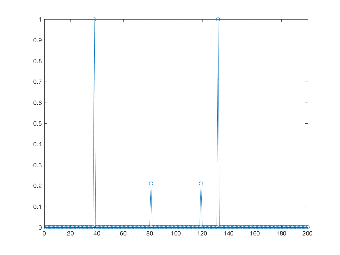
A plot of the lagrange multipliers is shown below. Notice that only three values are non-zero. These correspond to the support vectors.

I re-solved the problem with . The results are shown below. Notice that with less weight on keeping the errors small, a two of the samples fall into the margin area.

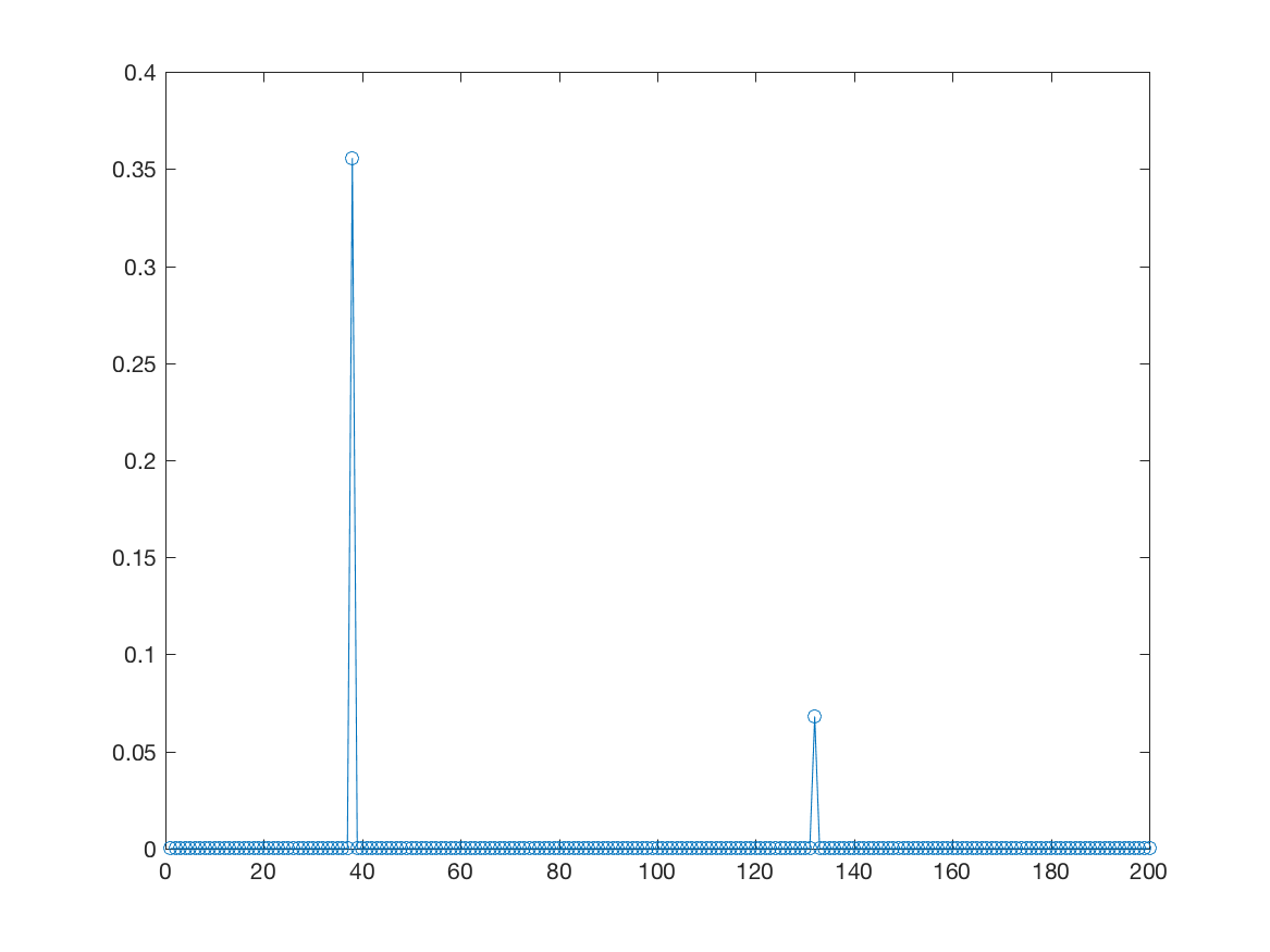
Here is a plot of the vector.
Here is a plot of the vector. The error is positive for those two samples that fall into the margin slab.
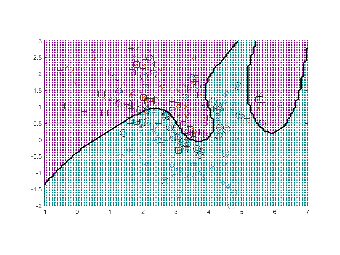
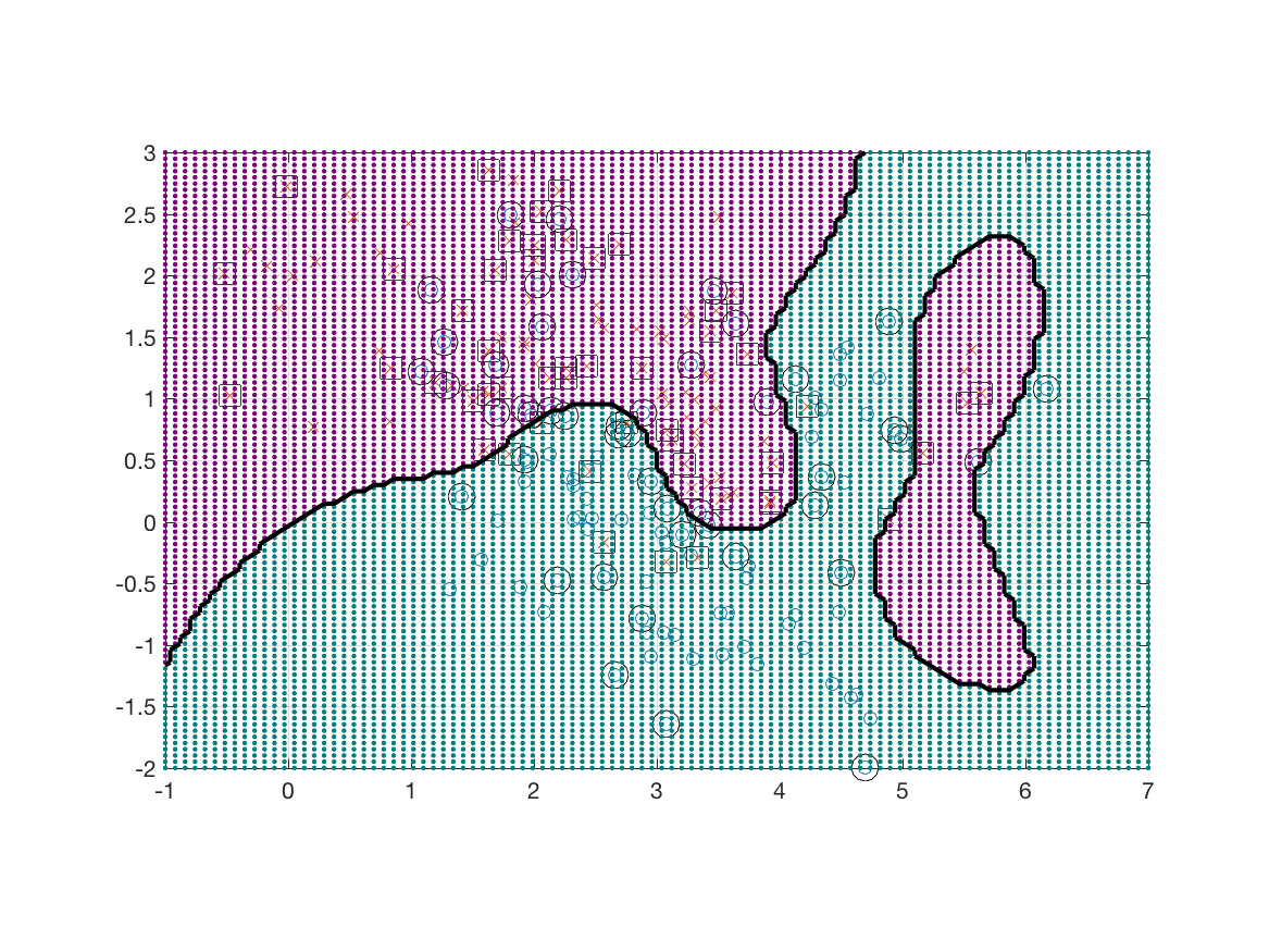
Next I loaded the mixture dataset and used the radial basis function kernel. The results for are shown below.
To prove that it is working, I evaluated the learned classifier at 10,000 test points and used color to encode the decisions in the figure below.
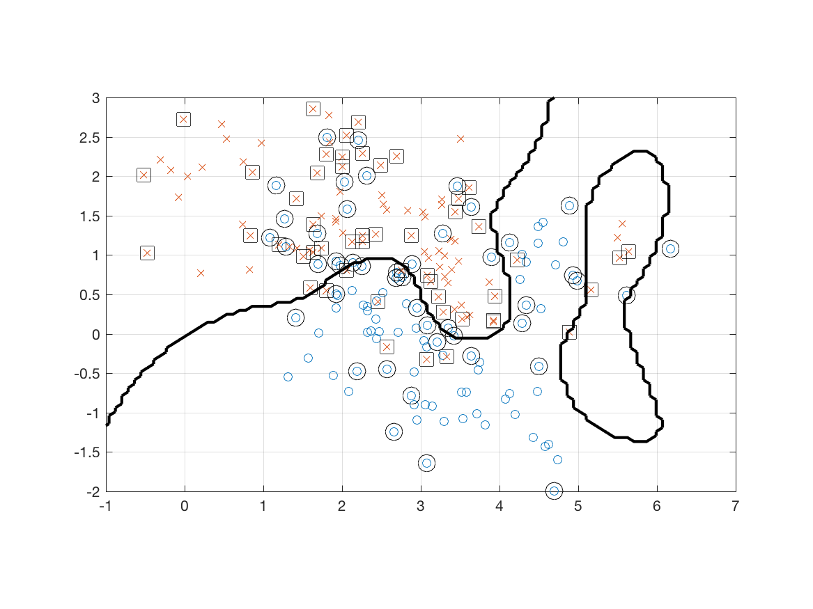
And here are the results when .
Here are 10,000 test points.