Signal Analysis in Matlab

Suppose you want to perform Fourier analysis of the sinc signal

$x(t) = \frac{\sin(2\pi F_0 t)}{\pi t}, -\infty < t < \infty,$

which has Fourier transform (CTFT) given by the rectangular function

$X(F) = \begin{cases} 1, & |F| < F_0, \\ 0, & \text{otherwise}. \end{cases}$

To perform the analysis you enter the following code into Matlab.

 
% SET SIGNAL PARAMETER AND SAMPLING RATE
F0 = 100; % [Hz], bandwidth of sinc function
Fs = 2000; % [Samples/second], sampling rate, need Fs > 2*F0 to avoid aliasing
% GENERATE TIME-DOMAIN SIGNAL
L = round((5*Fs)/(2*F0)); % width of time window
n = [-L:L]; % [samples], discrete-time index
t = n/Fs; % [seconds], vector of time samples
x = sin(2*pi*F0*t)./(pi*t); % evaluate sinc function
x(t==0) = 2*F0; % fix divide by zero in previous line
% COMPUTE FOURIER TRANSFORM
NFFT = 2^(nextpow2(length(n))+4); % choose the size of the FFT
f = [0:NFFT-1]/NFFT; % [cycles/sample], vector of discrete-time frequencies [0,1)
f = f - 0.5; % [cycles/sample], vector of discrete-time frequencies [-0.5,0.5)
F = f*Fs; % [Hz], vector of continuous-time frequencies [-Fs/2,Fs/2)
X = fft(x,NFFT); % compute Fourier transform, (frequency order [++++,----])
X = fftshift(X); % swap halves, (frequency order [----,++++])
% PLOTTING
subplot(211); plot(t,x); % plot the time-domain signal
grid on;
xlabel('Time [seconds]');
ylabel('Amplitude');
subplot(212); plot(F,abs(X)); % plot the Fourier transform
grid on; xlim(F0*[-3,3]);
xlabel('Frequency [Hz]');
ylabel('Magnitude');

This produces the plots below.

sig1

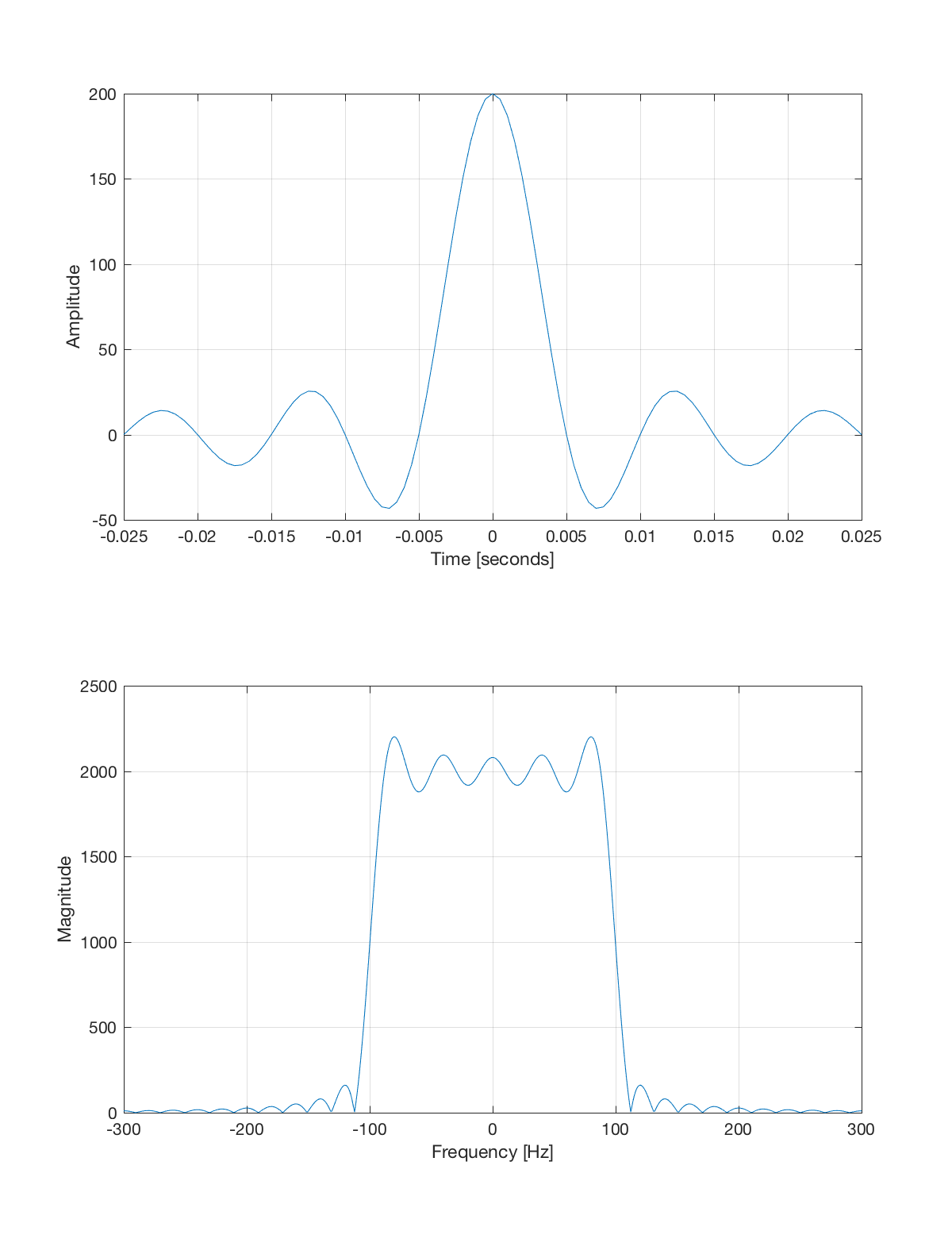
Is this the expected result?

Time-Domain Function. The sinc function has zero crossings when $2\pi F_0 t = \pi k$ for $k=\pm 1, \pm 2, \pm 3, \cdots.$ With the choice $F_0 = 100$ Hz, this leads to zero crossings a mutliples of $1/(2F_0) = 0.005$ and we see that this is indeed the case. The peak of the sinc function at $t=0$ should be $2F_0 = 200$ and we see that this is also the case. All the characteristics of the time-domain function $x(t)$ are as expected.

Frequency-Domain Function. The general shape of the Fourier transform approximates the rectangular pulse $X(f)$ . It "turns on" between $-F_0 = -100$ Hz and $F_0=100$ Hz as expected. But the shape is not quite right, and the magnitude is 2000, not 1 as expected. What is going on here?

Widowing. The distortion in the Fourier transform plot can be explained by recognizing that the Matlab code above does not compute the Fourier transform of $x(t)$ because it only evaluates $x(t)$ in the interval $-L/F_s \leq t \leq L/F_s,$ whereas $x(t)$ is defined on the entire set of real numbers $-\infty < t < \infty$ . What the code is really doing is computing the Fourier transform of the part of the signal snown above, i.e. it is computing

$\int_{-L/F_s}^{L/F_s} x(t) e^{-j2\pi F t} dt$

instead of

$X(f) = \int_{-\infty}^\infty x(t) e^{-j2\pi F t} dt.$

Another way of looking at this is to think of the Fourier plot above being the exact Fourier transform of a windowed version of $x(t)$ . Define a window function $w(t)$ as follows

$w(t) = \begin{cases} 1, & |t| \leq L/F_s, \\ 0, &\text{otherwise}\end{cases}$

and define $y(t) = w(t) x(t)$ to be the windowed signal. The Fourier plot shown above is $Y(F)$ . The ripples in $Y(F)$ are a mafestation of the Gibbs phenomenon. Another way explanation comes from the multiplication property of the Fourier transform. Multiplication of $w(t)$ and $x(t)$ in the time domain causes convolution of $W(F)$ and $X(F)$ in the frequency domain. When $X(F)$ , a rectangular function, is convolved with $W(F)$ , a sinc function, the result is a smearing of the rectangular function, and this is what we see in the figure above.

To make the windowed function $y(t)$ be a closer approximation of the true infintely long since function $x(t)$ , lengthen the window. The code above was modified by increasing the value of $L$ by a factor of 10 as shown in the code snipit below.

 
L = round((50*Fs)/(2*F0)); % width of time window

The new figures appear as shown below.

sig2

Notice that more of the sinc function is visible in the window. As a result, the Fourier transform of the windowed function is a closer approximation of the rectangular function, though the Gibbs phenomenon is still visible.

Any time a computer is used to compute the Fourier transform of an infinite length signal, windowing is inevitable. Therefore, the Fourier transforms will exhibit windowing effects which tend to smear sharp edges leaving behind Gibbs type effects near those frequencies.

Sampilng. While windowing explains the distortion of the shape of the Fourier transform, it does not explain the amplitude scaling. The amplitude of the Fourier transform is expected to be 1, but shows up as 2000. What causes this change in scale?

We should recognize that sampling is present in the Matlab code. The function $x(t)$ is not evaluated at every time $t$ , but only at a discrete set of times controlled by the sample rate $F_s$ . The signal generation code is repeated here for convenience.

 
% GENERATE TIME-DOMAIN SIGNAL
L = round((5*Fs)/(2*F0)); % width of time window
n = [-L:L]; % [samples], discrete-time index          <=== n is a list of integers
t = n/Fs; % [seconds], vector of time samples         <=== t is a scaled version of n
x = sin(2*pi*F0*t)./(pi*t); % evaluate sinc function  <=== evaluate at discrete times
x(t==0) = 2*F0; % fix divide by zero in previous line

Recall that sampling in the time domain corresponds to periodic replication in the frequency domain followed by amplitude scaling and scaling of the independent variable.

$x_d[n] = x_c(t) |_{t=nT} \qquad \text{(time-domain sampling)} \\ X_d(f) = F_s \sum_{k=-\infty}^\infty X_c\left([f-k]F_s\right) \qquad \text{(periodic replication)}$

Assuming the sample rate is chosen high enough $F_s > 2F_{\text{max}}$ , where $F_\text{max}$ is the highest frequency in $x_c(t)$ , the shifted replicas of $X_c(F)$ do not overlap and we have the relation

$X_d(f) = F_s X_c(f F_s), \qquad |f|\leq \frac{1}{2}.$

The difference between a discrete Fourier transform $X_d(f)$ computed by Matlab and the continuous-time Fourier trasnform $X(F)$ is a scale factor equal to the sample rate $F_s$ . In the example above, the sample rate is $F_s = 2000$ samples/second. This explains the scale factor observed in the figures above.

Summary. When performing signal analysis in Matlab, remember that windowing effects can alter the shape of signal spectra. Recognize that spectra of discrete-time signals are $F_s$ times higher than the corresponding continuous-time spectra.