Frequency Modulation (FM) Demodulation Lab

Objectives

1. Learn about FM and FM demodulation.
2. Learn about instantaneous frequency.
3. Practice designing filters and applying them to signals.
4. Practice using multi-rate processing (downsampling).

Introduction to FM and FM Demodulation

Let $x(t)$$x(t)$ be the real-valued message signal which could represent speech or music. Frequency modulation (FM) encodes the message into the instantaneous frequency of the modulated/transmitted (TX) signal $y_{\text{TX}}(t)$$y_\text{TX}(t)$ which has the form

where $F_c$$F_c$ is the carrier frequency and $k$$k$ is a constant. The function $\phi (t)$$\varphi(t)$ is the phase function. The instantaneous frequency $F_i(t)$$F_i(t)$ of any sinusoidal wave is the derivative of its phase function

We see that for FM, the instantaneous frequency is a constant (the carrier frequency $F_c$$F_c$) plus a scaled version of the message $x(t)$$x(t)$.

A radio antenna will pick up all the FM signals that are transmitted in the area. The received signal (RX) has the form

Each received FM signal will have a different amplitude $A_m$$A_m$, phase ${\theta }_m$$\theta_m$, carrier frequency $F_{c,m}$$F_{c,m}$, and message $x_m(t)$$x_m(t)$. In the United States, carrier frequencies start at 88.1 MHz and end at 107.9 MHz with 200 kHz spacing, which provides 100 unique FM stations. FM carrier frequencies are 88.1, 88.3, 88.5, 88.7, 88.9, 89.1, ..., 107.5, 107.7, 107.9 MHz. Notice that all valid carrier frequencies end in odd-tenths. This page shows the FM spectrum on the USU campus (at the moment I recorded it). Because each FM broadcaster in any given area uses a different carrier frequency, the signal you want to listen to can be isolated from the others using a bandpass selection filter. The isolated signal of interest has the form

where the subscripts have been dropped. This signal is mixed with $\cos$$\cos$ and $\sin$$\sin$ at the carrier frequency $F_c$$F_c$ to bring the signal to baseband. This is an application of the frequency-shifting property of the DTFT. If we treat the $\cos$$\cos$ and $\sin$$\sin$ branches of the receiver as the real and imaginary parts of a complex-valued signal, that signal takes the form

This is called the "complex-baseband" form or "complex envelope" because the signal is expressed as a complex exponential signal and the carrier frequency has been removed, i.e. it is centered at zero frequency also known as baseband, zero frequency, or DC. We can use the complex-baseband form to discuss demodulation which is the process of recovering $x(t)$$x(t)$.

How can $x(t)$$x(t)$ be extracted from inside the complex-exponential and the integral? Let's try taking the derivative of $y(t)$$y(t)$. This requires use of the chain rule and Leibniz integral rule. The answer is

The derivative brings $x(t)$$x(t)$ out side both the exponential function and the integral. The message $x(t)$$x(t)$ now acts like amplitude modulation. The complex exponential can be canceled by multiplying by the conjugage of $y(t)$$y(t)$

Finally, if we take the imaginary part of $z(t)$$z(t)$, we recover a scaled version of $x(t)$$x(t)$ which was our goal.

In summary, the sequency of operations in receiving and demodulating FM are as follows.

1. Mix the signal of interest to baseband by multiplying by $\exp (-j2\pi F_{c}t)$$\exp(-j2\pi F_c t)$.
2. Apply a low-pass filter to isolate the signal of interest and remove all the other signals resulting in the complex-baseband signal.
3. Differentiate the complex-baseband signal (using a differentiating filter) and multiply by the conjugate of the complex-baseband signal.
4. Take the imaginary part resulting in an audio signal.

All of these steps may be performed in about five lines of Matlab code. Along the way, the sample rate must be reduced so that the samples can be fed to a sound card. This involves downsampling which we stuied in a previous lab assignment.

Let's Do It!

1. Download the signal fm_rds_2400k_complex2. This file is almost 400 MB. (Special thanks to John E. Post for the data and his article entitled "FM RECEPTION WITH THE GNU RADIO COMPANION" which gives a lot of good information about FM and includes links at the end of the article to other reference material.)

2. Read some of the signal into into the Matlab workspace. Here's a few things to keep in mind from the datafile web page.

   1. The sample rate of the data is $F_s=2.4$$F_s = 2.4$ MS/s.
   2. The data was captured with a receiver tuned to 106.7 MHz as it's center frequency.
   3. GnuRadio software was used in the data capture. GnuRadio stores the in-phase (real) and quadrature (imaginary) samples in interleaved order using 32-bit floating point type.

Fs = 2.4e6; % [samples/second] = sample rate (given on web page and in filename)
Fc = 106.7e6; % [Hz] = center frequency (given on web page)
Nsec = 5; % [seconds] = number of seconds of data to read in
Ns = Nsec*Fs; % Number of samples to read in
fid = fopen('fm_rds_2400k_complex2','rb'); % Open the file
x = fread(fid,2*1e5,'float'); % Toss first 10^5 samples (they can have unwanted transients)
x = fread(fid,2*Ns,'float'); % Read in the samples you want
fclose(fid); % Close the file
x = complex(x(1:2:end),x(2:2:end)); % Convert to complex I/Q

3. When you meet a new signal, it's a good idea to visualize it in the time domain, frequency domain, and/or in time-frequency space using a spectrogram. In this part, make two spectral plots of the given signal. In one plot, use a true scaled frequency axis. In the second plot, use a normalized frequency axis. Here is some basic Matlab code showing how to do this and the plots follow.

xxxxxxxxxx
NFFT = 2^18; % FFT size, this may not be all the data and that's ok
fx = [0:NFFT-1]/NFFT - 0.5; % Normalized frequency (if NFFT is an even number)
Fx = fx*Fs + Fc; % True frequencies in Hz
X = abs(fftshift(fft(x,NFFT))); % Compute the spectrum
subplot(211); plot(Fx/1e6,20*log10(X)); % Plot in MHz
subplot(212); plot(fx,20*log10(X)); % Plot in normalized frequency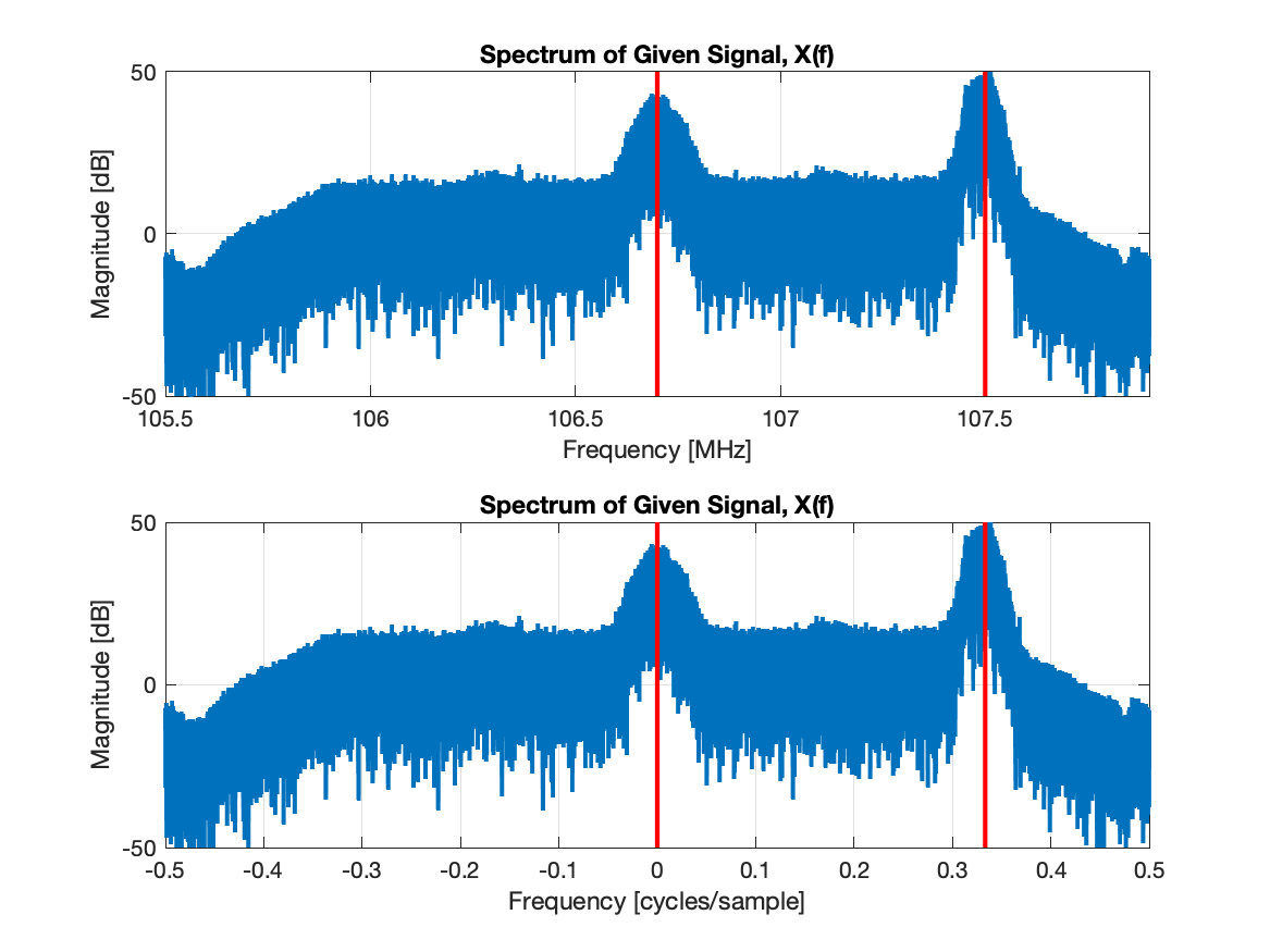

These spectral plots reveal that there are actually two FM signals picked up in the 2.4 MHz bandwidth of the received signal. The red-lines mark the carrier frequencies which are 106.7 MHz and 107.5 MHz. We can see that each of the FM signals has a bandwidth of 200 kHz centered on the carrier frequency.

The lower spectral plot uses normalized frequency to show where the signals actually are in the data. This plot shows that one of the FM signals is already at baseband (zero frequency) while the other one is at (107.5 - 106.7)/2.4 = 0.8/2.4 = 1/3 = 0.3333 cycles/sample.

4. We will demodulate the signal that appears at baseband. If we wanted to demodulate another signal, we just have to move it to baseband by mixing with (multiplication by) a complex exponential $\exp (-j2\pi f_{\mathrm{\Delta }}n)$$\exp(-j2\pi f_\Delta n)$, where $f_{\mathrm{\Delta }}$$f_\Delta$ is the desired amount of shift. A property of the DTFT predicts that mixing with a complex exponential signal causes a frequency shift, and the pictures below indicate that is exactly what happens when $f_{\mathrm{\Delta }}=1/3$$f_\Delta = 1/3$. Notice that the signal at 107.5 MHz now appears at baseband. Try this yourself and make spectral plots of the frequency shifted spectra.

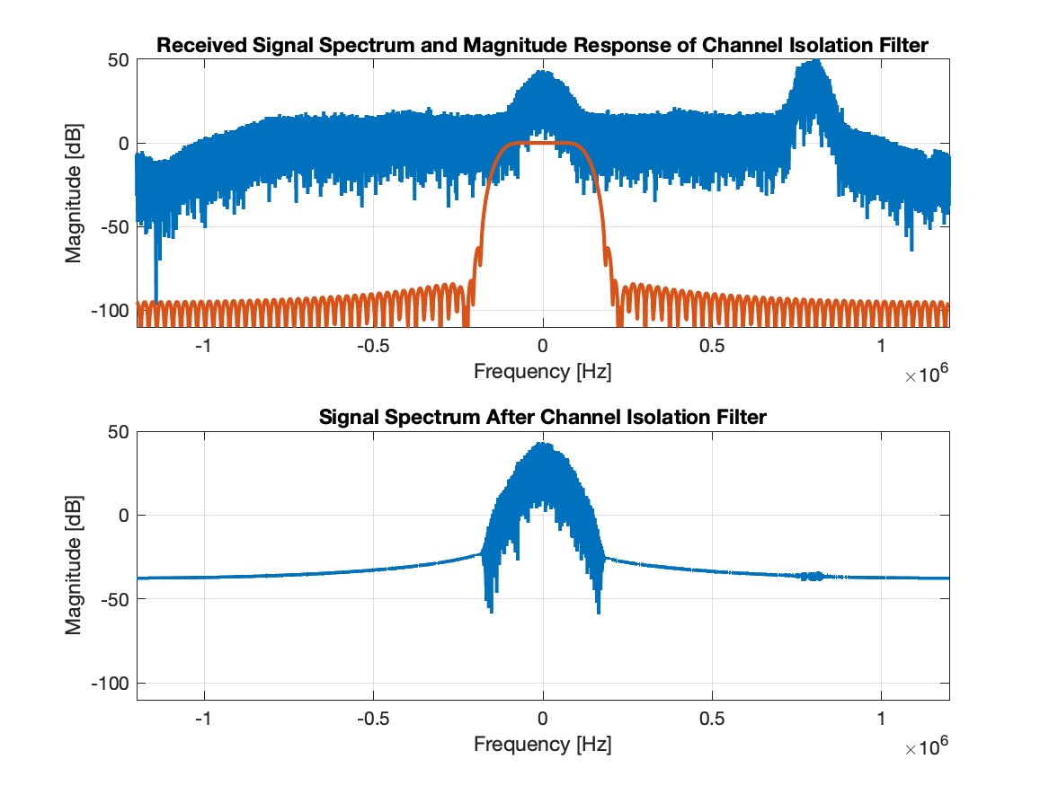
5. The first step in demodulating an FM signal is to isolate it from other signals that may be present. To accomplish this, we will use a low pass filter. The filter should pass the signal of interest which extends to $F_{\text{pass}}=100$$F_\text{pass} = 100$ kHz above the carrier and stop other signals. Let's let $F_{\text{stop}}=150$$F_\text{stop} = 150$ kHz. Normalize these frequencies by the sample rate $F_s=2.4$$F_s = 2.4$ MHz and design a trapazoidal filter with a Hamming window. Then apply it to the signal. When I did this, I obtained the following plots which show (upper) the spectrum of the original signal and the magnitude response of the LPF. The lower plot shows the spectrum of the filtered signal which contains the FM signal of interest and the other FM signal has been removed.

6. All that empty spectral space indicates that the signal is now oversampled and may be compressed/decimated without loosing any information. Compressing/decimating the signal will expand it in the frequency domain. How much can the signal be expanded in the frequency domain? The highest frequency in the filtered signal is about 200 kHz and the highest frequency representable is 1.2 MHz which is half the sample rate 2.4 MHz. Taking the ratio gives 1.2 MHz/200 kHz = 6. We can decimate the signal as follows.

xxxxxxxxxx
D = 6; % Decimation factor
Fs = Fs/D; % Reduce the sample rate
yd = ylpf(1:D:end); % Compress in the time domain causes expansion in the frequency domain

Perform these steps and then make spectral plots of the signal before and after compression/decimation. Use a normalized frequency axis. Here's what I got.

The compression step is not absolutely necessary but it reduces the amount of data for subsequent processing. Thus compression when possible makes for efficient processing. The sample rate has to be reduced at some point because the result of demodulation is audio data and most sound cards require sample rate below 100 kS/s. Compressing by a factor of D=6 leads to a sample rate of 2.4e6/6 = 400 kS/s. Some additional compression will be needed in a later step.

Before proceeding any further it's worth pausing to look at the spectrogram of the signal before the compression step. A short segment of that spectrogram is shown below. Remember that a spectrogram, when viewed as an image, shows how the frequency of the signal varies over time. Also remember that in FM, the message $x(t)$$x(t)$ is encoded in the frequency of the signal. Therefore, by looking at the spectrogram, you can actually see the message signal $x(t)$$x(t)$! Demodulation is the process of extracting what we can already see in the spectrogram.

7. The next step in FM democulation is differentiating the signal. There's two things that we need to keep in mind: (1) we differentiate the signal using a filter, and (2) that derivative filter causes a delay. The delay is not bad, but remember that the next step is to multiply the output of the derivative filter by the conjugate of the input of the derivative filter. Remember the step $z(t)=y^{\ast }(t)(dy(t)/dt)$$z(t) = y^\ast(t) (d y(t)/ dt)$. It's vitally important that we keep our signals time aligned. If the derivative signal $dy(t)/dt$$dy(t)/dt$ has been delayed by the action of filtering, then we must also delay $y^{\ast }(t)$$y^\ast(t)$ by the same amount. If we do this, then the signals will be time aligned and everything will work out. So we are going to design two filters: (1) a derivative filter, and (2) an all pass filter having the same delay as the derivative filter. Let's start with the derivative filter.

Recall the following property of the continuous-time Fourier transform.

In other words, a filter that differentiates a signal has frequency response given by $H(F)=j2\pi F$$H(F) = j2\pi F$. There's really no such thing as a derivative on a discrete-time signal, but we can design a filter having a frequency response given by $H(f)=j2\pi f$$H(f) = j2\pi f$. The impulse response of such a filter is

Derive this result and include this in your report. Here are a few ideas to get started. We want to perform a differentiation operation using a filter. The filtering property of the CTFT is:

So we see that if we let $H(F)=j2\pi F$$H(F) = j2\pi F$, then the result of convolution will be the derivative. Now there is no such thing as a derivative in discrete time, but taking inspiration from the continuous time case, we can design a discrete-time filter with frequency response $H(f)=j2\pi f$$H(f) = j2\pi f$ for $-\frac{1}{2}\le f<\frac{1}{2}$$-\frac{1}{2} \leq f < \frac{1}{2}$. The impulse response of this filter is given by

Now use integration by parts to find $h[n]$$h[n]$.

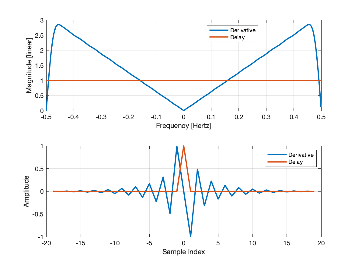
This IIR filter is not causal or stable, but we can build a causal, stable, FIR approximation by truncating this impulse response and delaying it. See the Matlab code below which also includes a Hamming window.

​x
% Design derivative and delay filter
L = 19; % Filter delay
n = [-L:L].'; % Time vector
deriv = (-1).^n ./ n; % Derivative filter impulse response
deriv(L+1) = 0; % Fix the zero in the center
deriv = deriv.*hamming(2*L+1); % Include the Hamming window
delay = zeros(2*L+1,1); % Make a delay filter
delay(L+1) = 1; % Set the delay

% Demodulate FM (in one line of code!)
z = conj(conv(yd,delay)) .* conv(yd,deriv);

Make a plot of the magnitude responses of the derivative and delay filters. Also make a plot of the impulse responses. Note that the magnitude response of the derivative filter is $|H(f)|=2\pi |f|$$|H(f)|=2\pi |f|$, i.e. it is an absolute value function.

8. Demodulate the FM signal using the Matlab code below

xxxxxxxxxx
% Demodulate FM (in one line of code!)
z = conj(conv(yd,delay)) .* conv(yd,deriv);

The demodulated signal has several components as shown in the figure below.

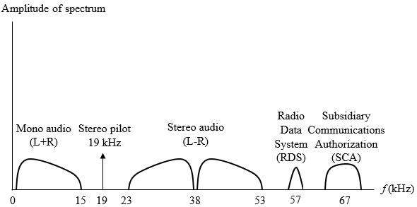
We want to extract just the left+right audio between 0 and 15 kHz using a low pass filter. Design a trapazoidal LPF. Make sure the filter passes the signal of interest and rejects everything at and above 19 kHz.

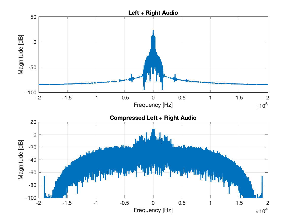
Apply the filter to the demodulated signal. Make two spectral plots. In the first one, show the spectrum of the demodulated FM signal and the magnitude response of your LPF. In the second plot, show the spectrum of the filtered signal. Here are my plots.

9. All that empty spectral space indicates that the filtered signal can be compressed/decimated without loss of information. As noted earlier, compression in the time domain causes expansion in the frequency domain. How much can the signal spectrum be expanded? The highest frequency is about 20 kHz and the higest representable frequency is 200 kHz which is half the sample rate. The ratio is 200 kHz / 20 kHz = 10. Thus we can compress/decimate the signal by a factor of $D=10$$D=10$. This reduces the sample rate to 400 kS/s / 10 = 40 kS/s. This is a low enough sample rate that we can pass the samples to an audio soundcard.

Compress the signal and make spectral plots before and after compression.

10. Take the imaginary part of the compressed signal and listen to it. Can you hear the message? Describe what you hear?
11. The given signal contains two FM signals. Shift the other signal to baseband and repeat the processing steps. Listen to that signal. Describe what you hear?

Report

Your report should include the code, plots, and derivation from the steps listed above.